Tutorials

Reviewer Notes

In this pre-release phase, GLIG reviewers should please add comments and changes to those already listed below.

1. File open and save dialogs should remember the last location used
2. If the user has saved project to a specific name, that one should be used instead of home
3. Project should save the nearby object, ground slope, flash density and line length data from the Phase View
4. Project should save the critical current simulation setup data.
5. Add Resistor tab to the Simplified interface; it’s commonly used to connect shield wires
6. Pre-fill the default LPM parameters for KI and E0
7. Pre-fill the default Ground parameters for E0
8. In the setup for critical current iterations, the prompts for first tower, last tower, and wire flags need to remain visible
9. On the ground tab, the formula behind *Get R60* should update to Dwight’s formula, because we changed the counterpoise ladder assembly.
   1. Dwight
   2. Note: Sunde’s is used in [1]:
10. Add guidance for determining tower inductance.
11. Python “hangs” when calculating flashover rate with line arresters.
12. When there are only 4 conductors, make S2 coordinates the same as S1 after clicking “Update coordinates” in the phase view.
13. Prefill the default Arrbez parameter for the reference voltage, and change units from “V” to “pu”.

500-kV Horizontal Line

This example is based on pp. 27-32 in Annex B of [1]. When you start the GUI, two windows appear. One is the main component panel called *OpenETran*, and the other is the *Phase View*.

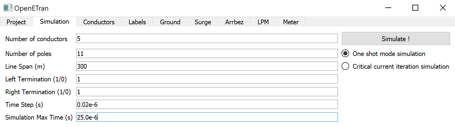
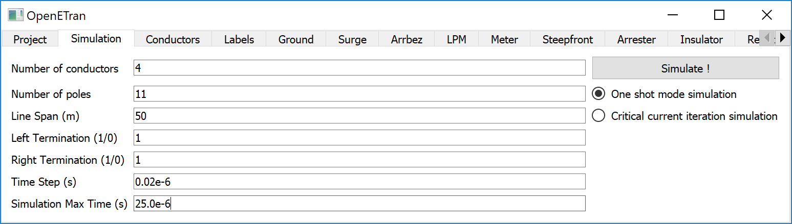
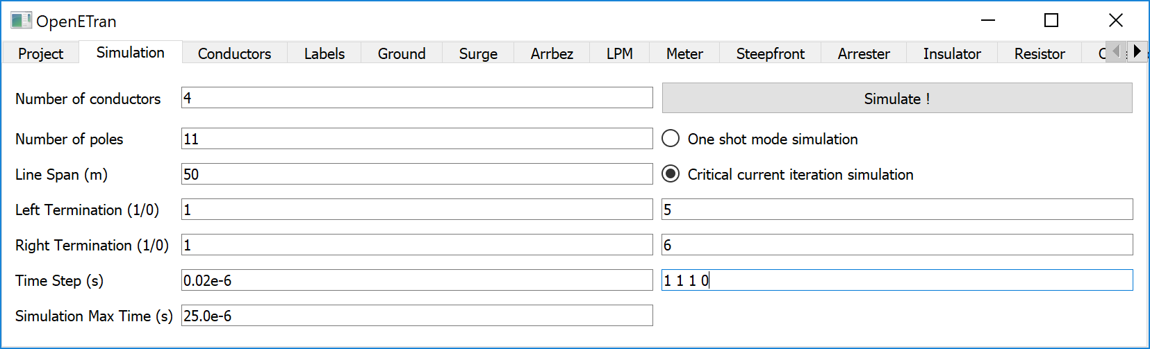
Click the *Simulation* tab on the main window and fill it out as follows. This creates a framework of 11 towers, each separated by 300 m. There are 5 conductors, to be labeled A, B, C, S1 and S2.

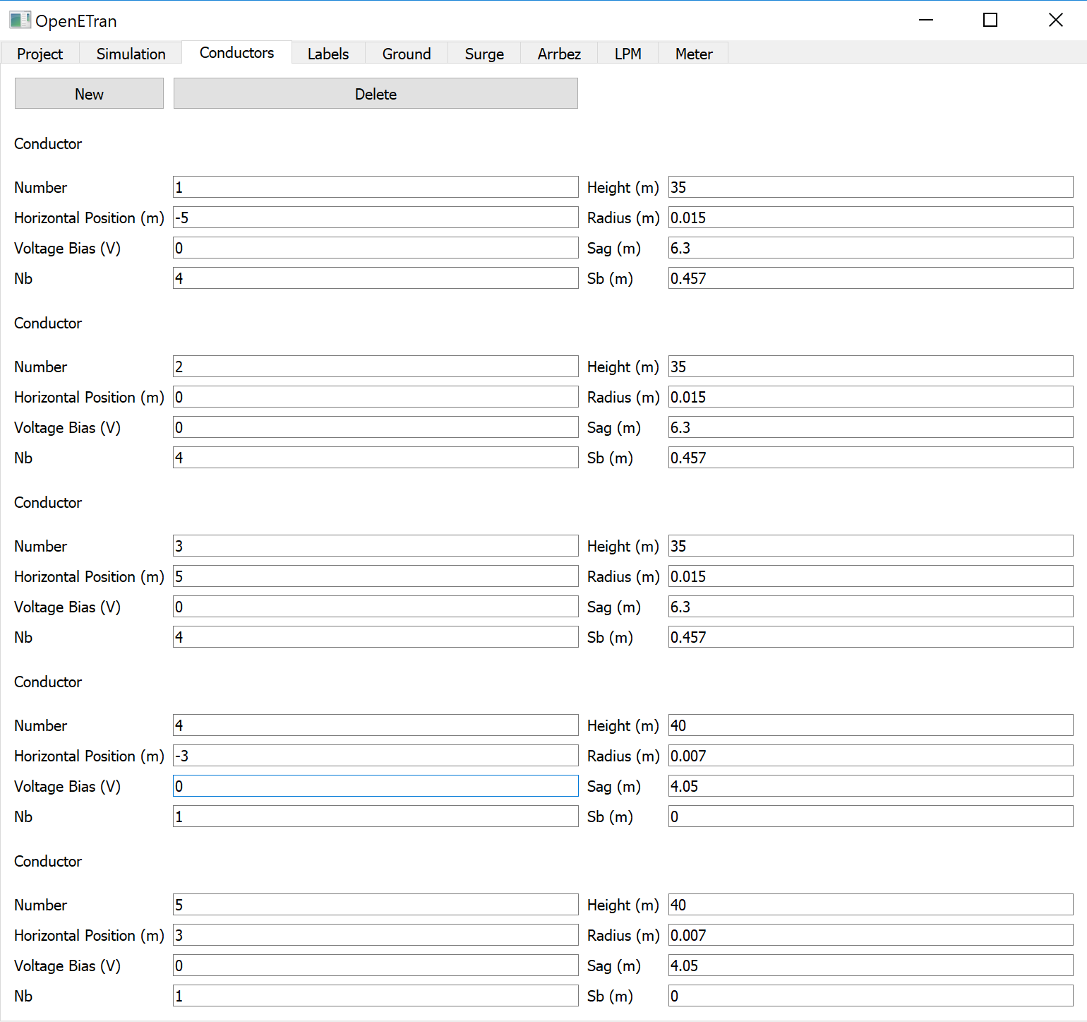
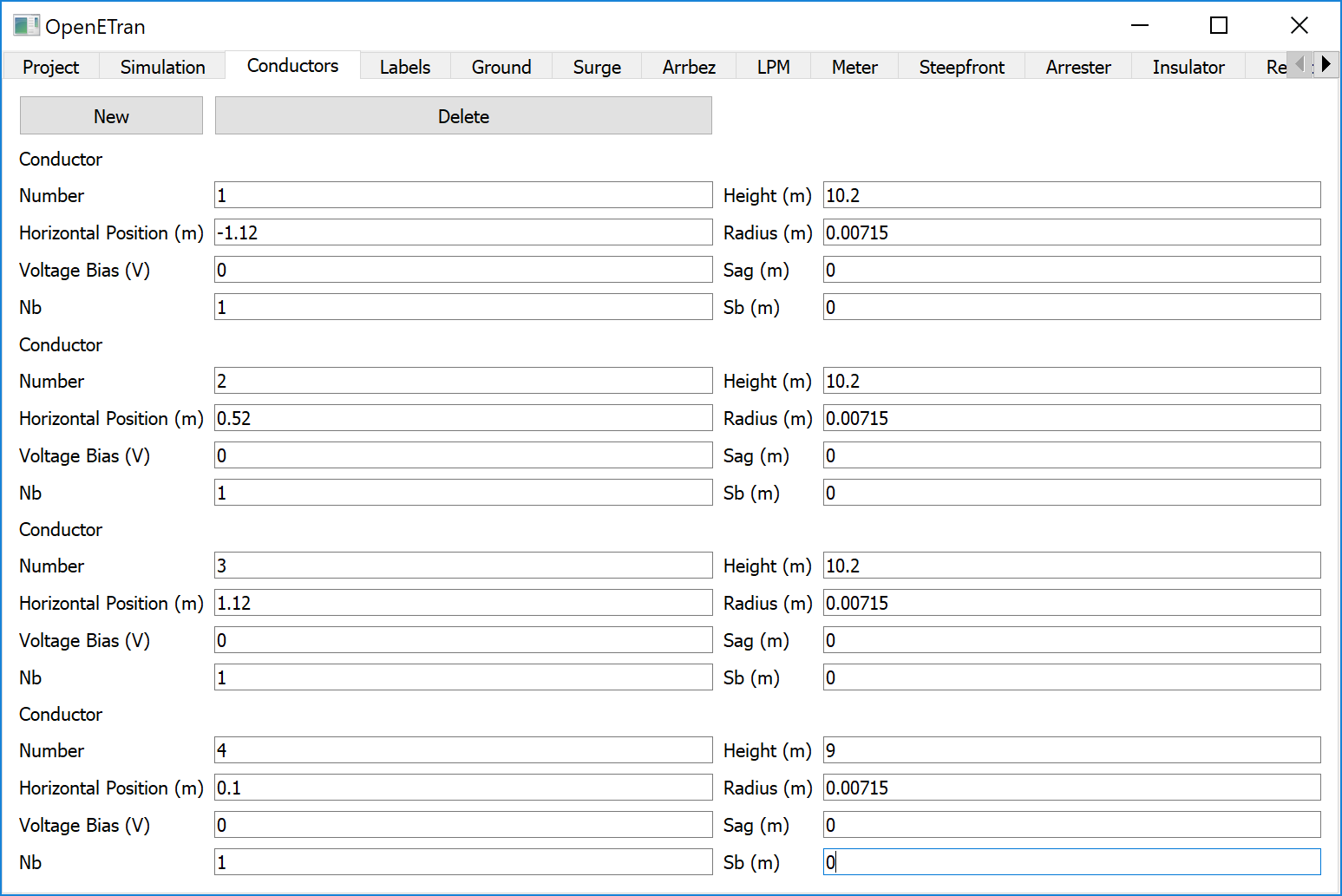
Click the *Conductors* tab, then click *New* four times, and fill it out as follows:

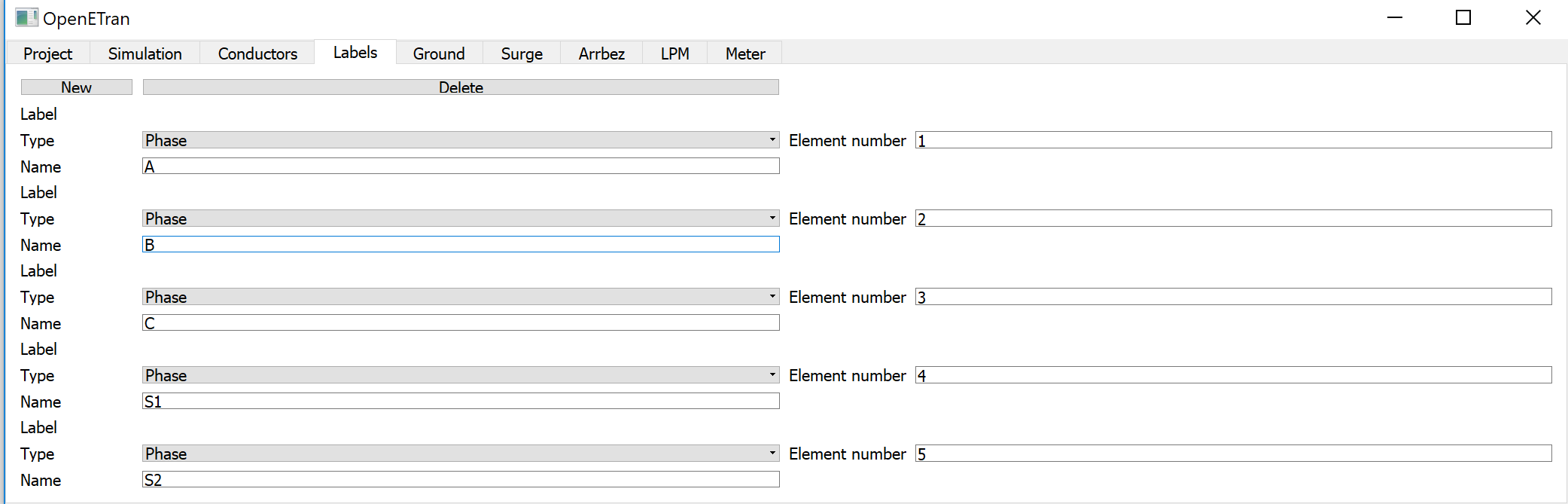
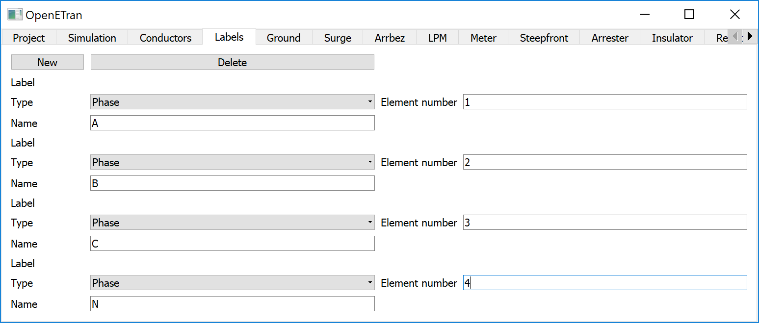
Click the *Labels* tab, then click *New* four times, and fill it out as follows:

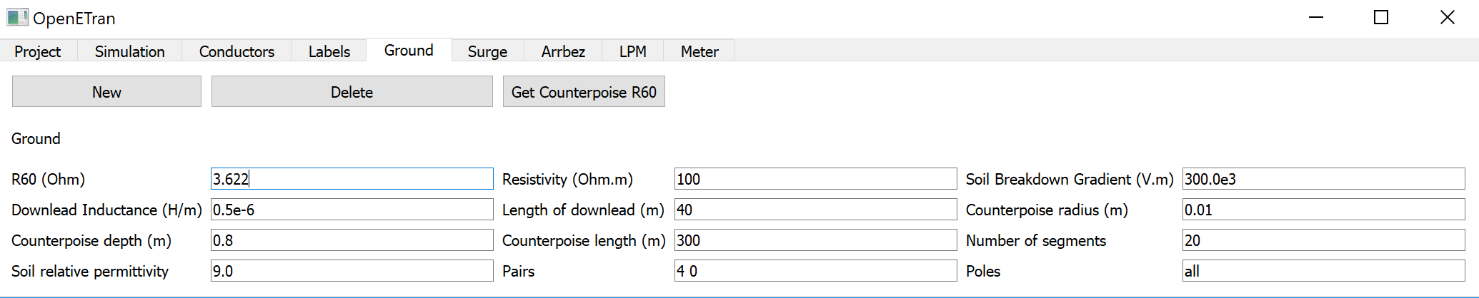
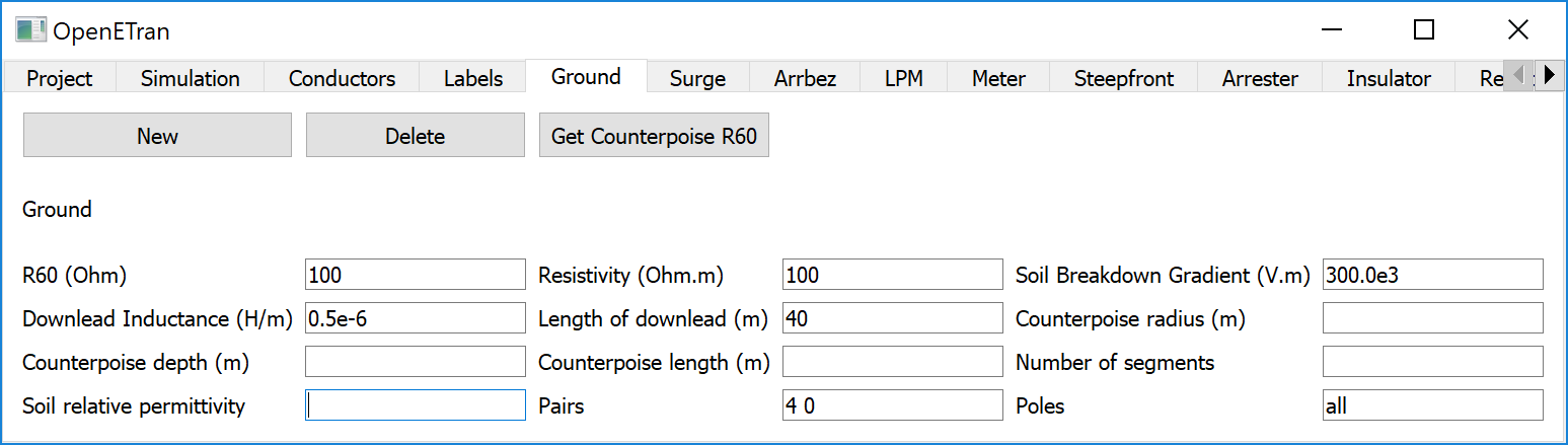
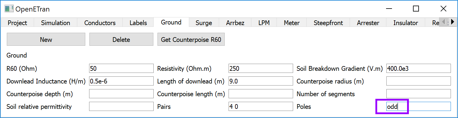
Click the *Ground* tab, and fill it out as follows. This puts a counterpoise and tower inductance on the first shield wire, S1, at every tower. We’ll connect S2 to ground later.

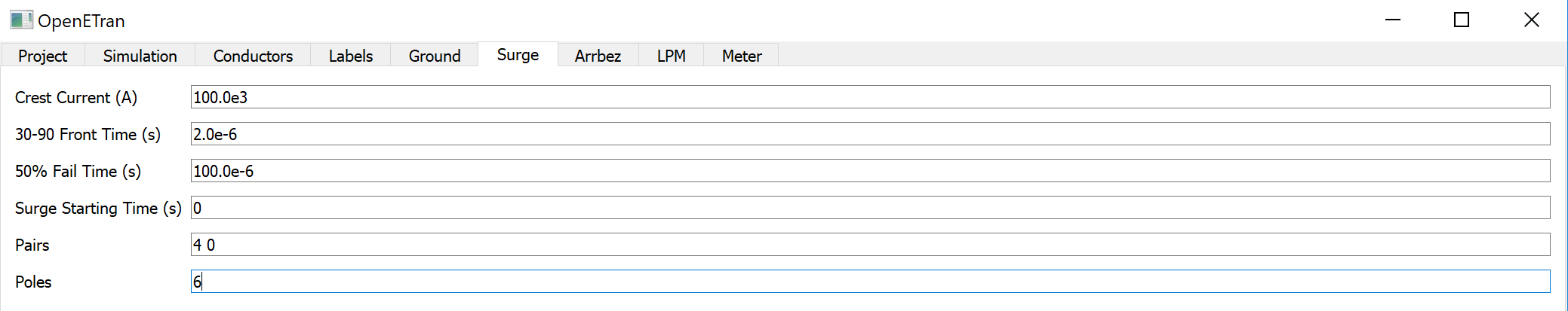
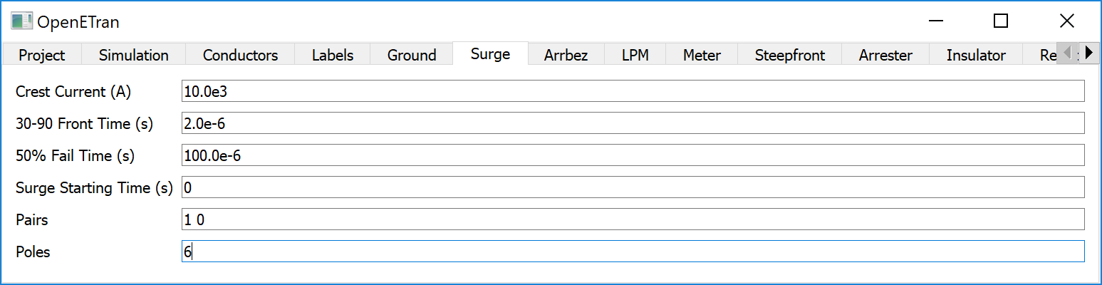
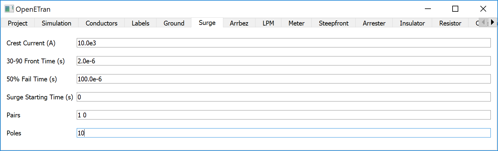
Click the *Surge* tab, and fill it out as follows. This puts a stroke to S1 of the middle tower.

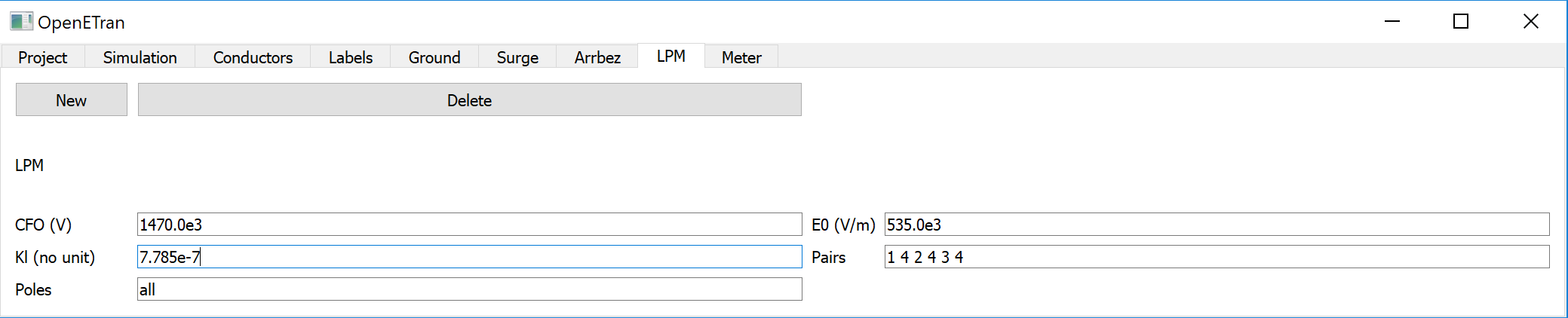
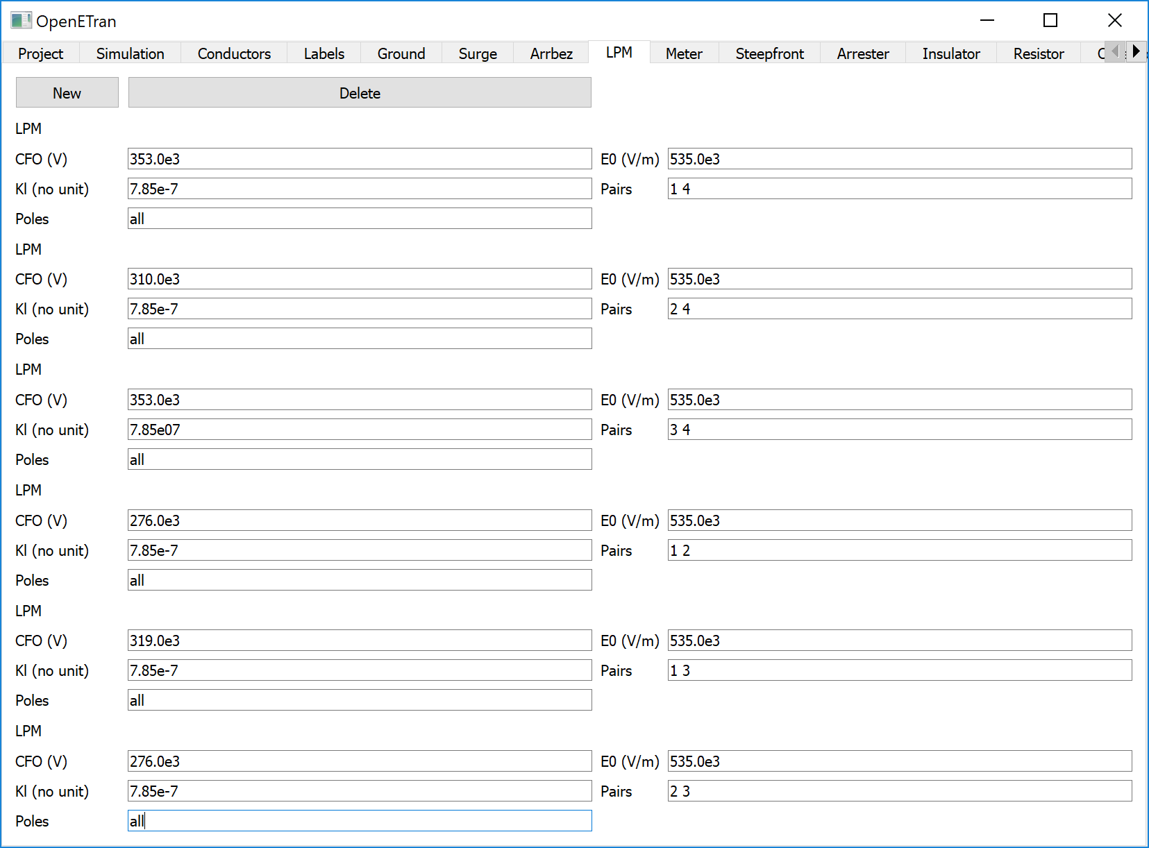
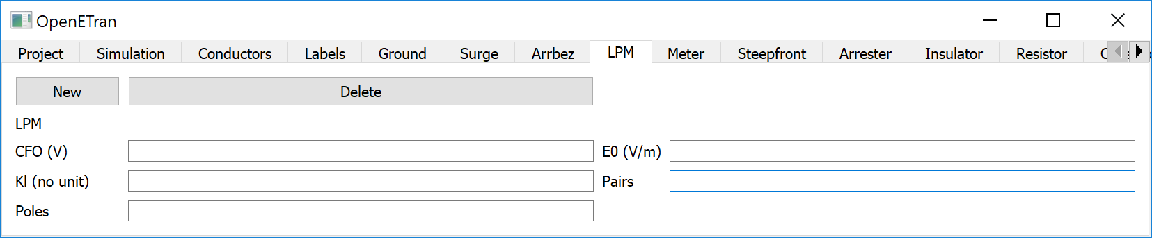
Click the *LPM* tab, and fill it out as follows. This puts insulation of 1470-kV CFO (i.e. strike distance over insulators of 3 m) on each phase. Time-dependence is represented in default parameters for the leader progression model.

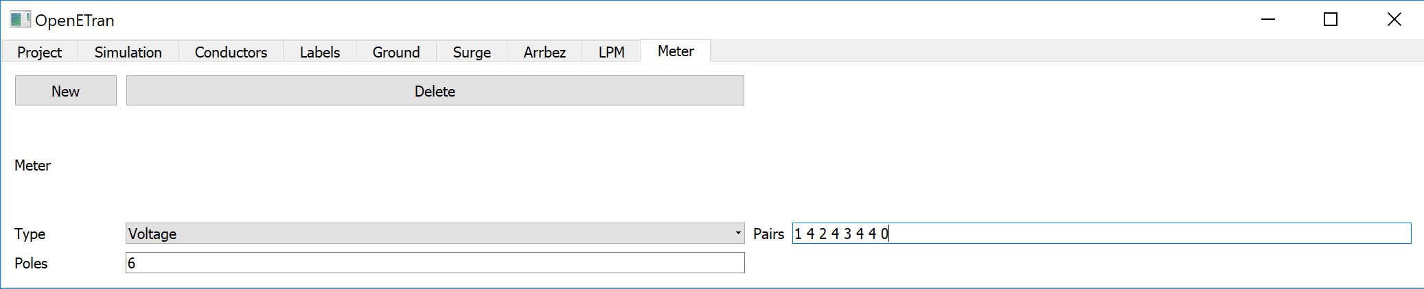
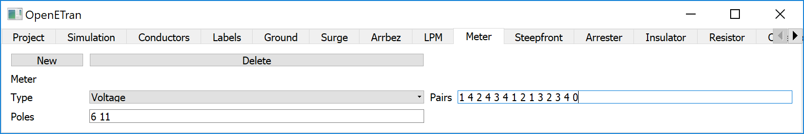
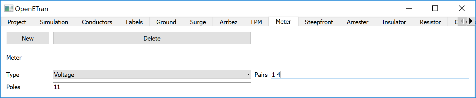
Click the *Meter* tab, and fill it out as follows. This requests voltage plots across each phase insulator, and from tower top to remote ground, just at the struck tower #6, which is the middle one of 11 towers.

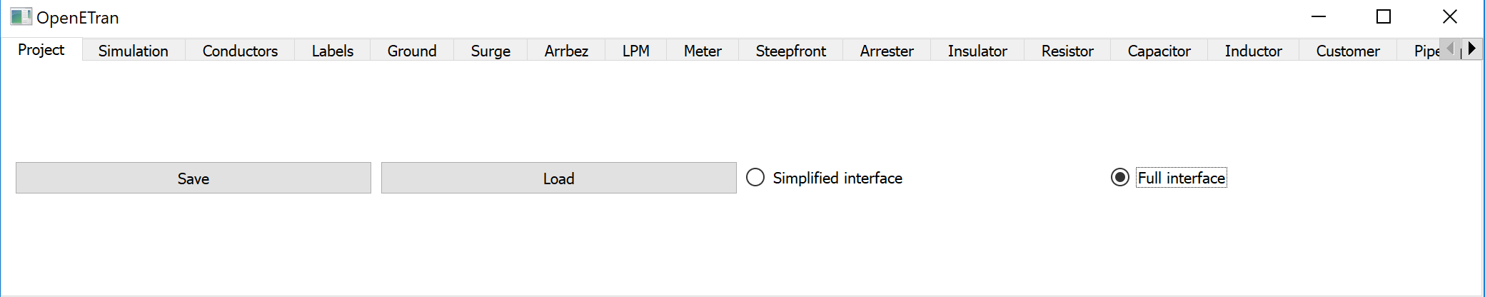
We’re not using line arresters now, but we still need to connect S1 and S2 at all towers. Go back to the *Project* tab and request the *Full Interface* by clicking the radio button.

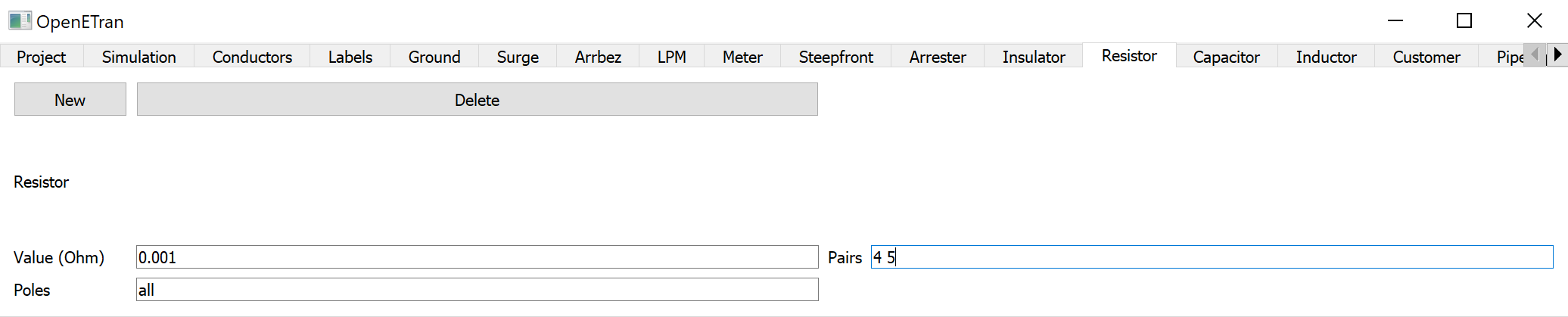
Click the *Resistor* tab and fill it out as follows. This 1-mΩ resistor connects S1 and S2.

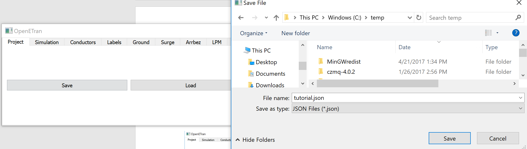
This is a good time to save your work, i.e. before attempting your first simulation. Click the *Project* tab again, Click the *Save* button and save the project to a file name and path of your choice.

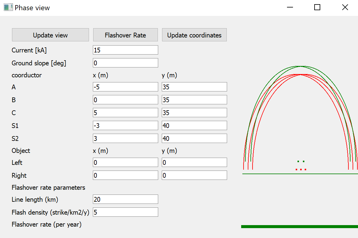
Now find the *Phase View* window and click *Update Coordinates*. It should now show your input conductor coordinates at the tower. This line is not perfectly shielded at 15 kA, as indicated by some exposure of the red arcs outside the green shielding envelope. Our critical current for shielding failures is yet to be determined; it may not be 15 kA.

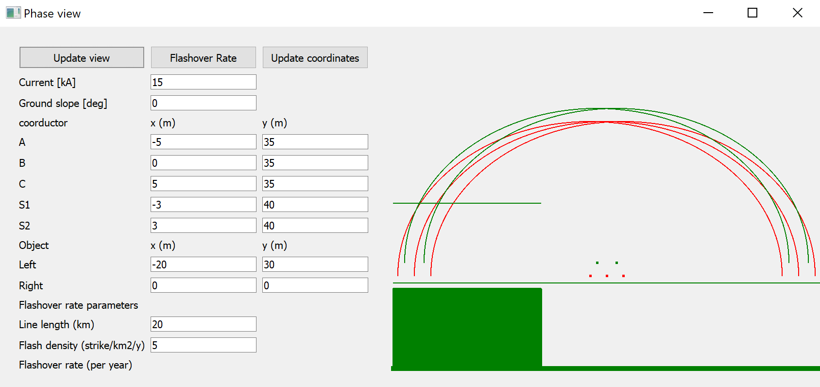
For illustrative purposes, put a tree line on the left-hand side of the line. Change the *Object Left* x and y coordinates to -20 and 30, respectively, then click *Update view.* Now the left side is shielded from strokes 15 kA or greater.

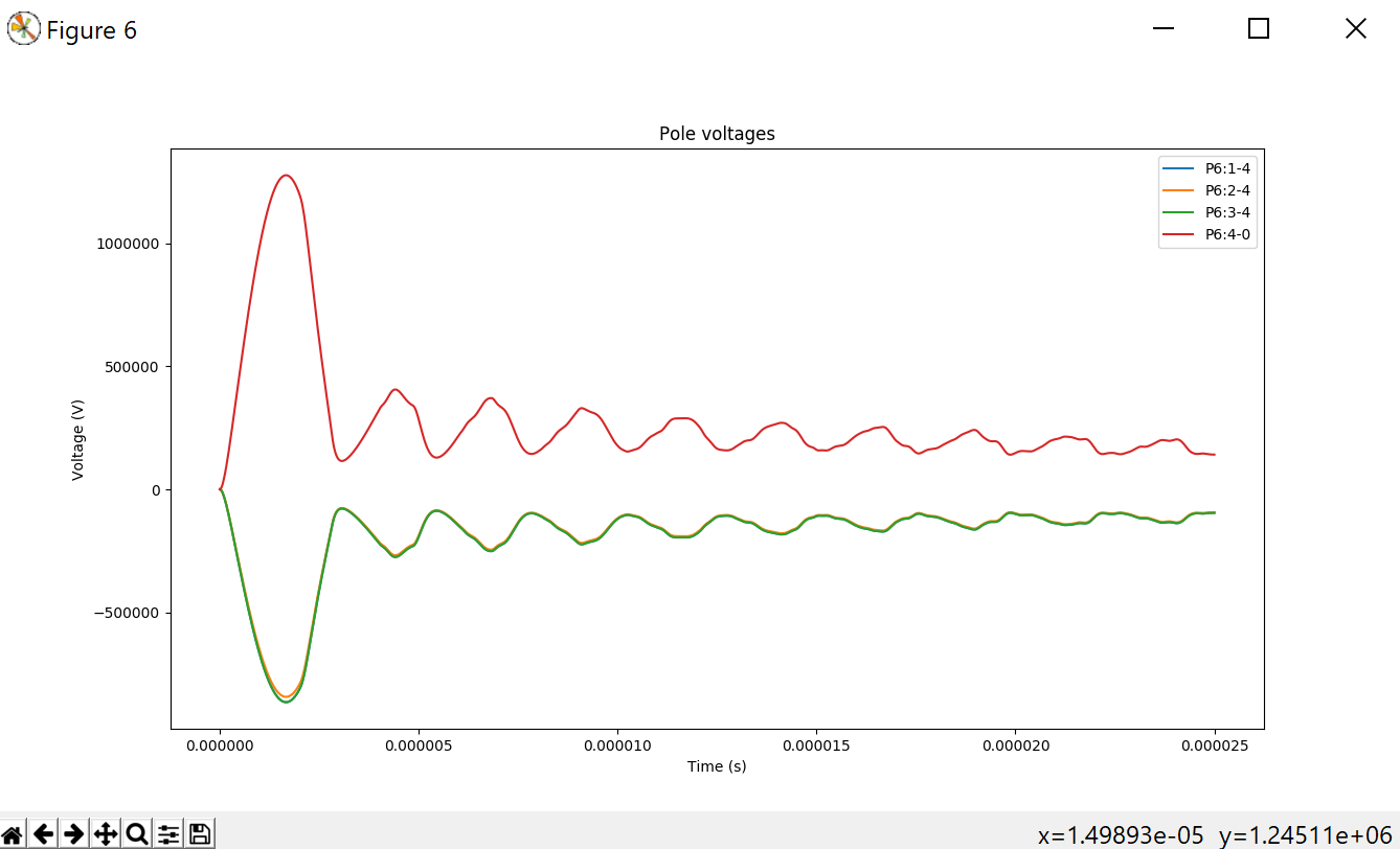
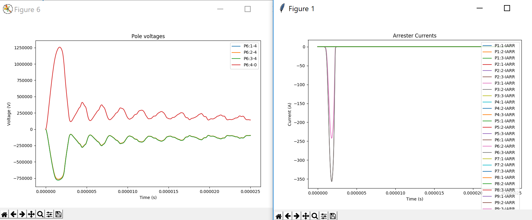
Back on the *OpenETran* window, click *Simulate* and then the *Simulate!* Button. After a couple of seconds, you see the following requested voltage plots at tower 6 for a 100-kA stroke. The peak tower voltage is about 1280 kV. It’s higher than 3.622 Ω x 100 kA, due to tower inductance and nonlinear frequency dependence in the counterpoise. However, the worst peak insulator voltages are -865 kV on the two outer phases, less than the 1470-kV CFO, so flashover would not be expected. Plot data was saved in a CSV file if you wish to do further processing in a program like Excel or MATLAB.

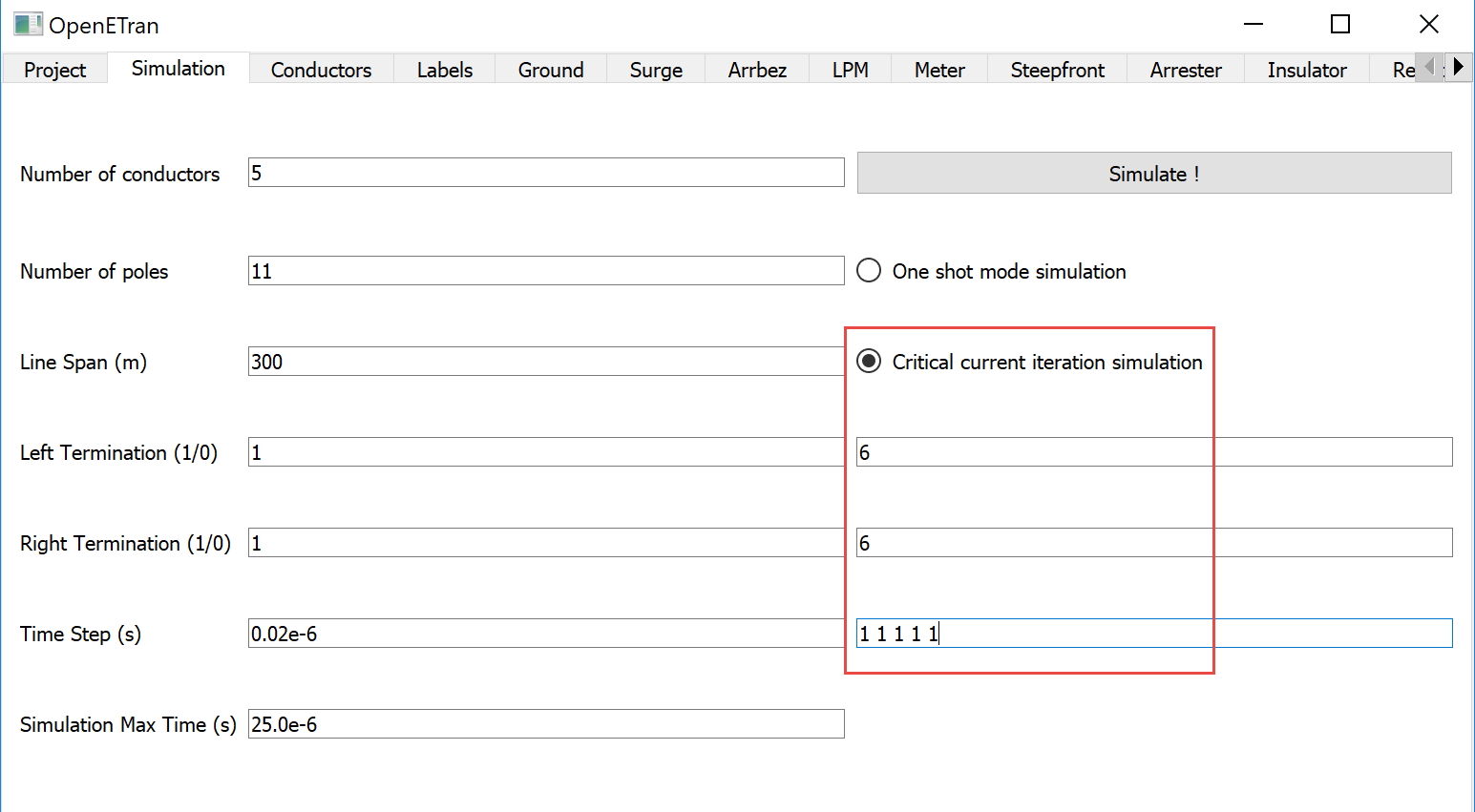
Close the plot window using the *X* in its upper right corner. Back *OpenETran* window, change the simulation control parameters as shown in the red highlighted area. This will run the program to determine critical currents, which just barely cause flashover, to any of the five conductors if struck at tower 6. You need to click the radio button for “Critical current iteration simulation” to see three additional input fields, each of which contains an input prompt. When ready, click the *Simulate!* Button.

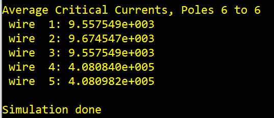
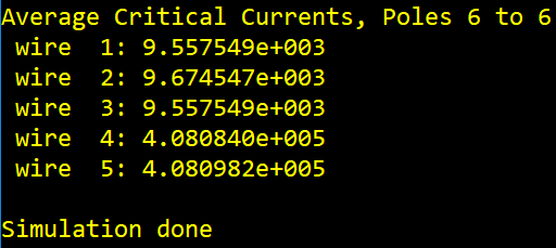
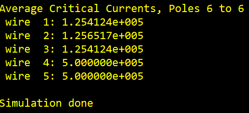
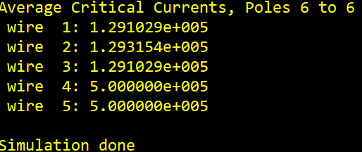
Within a few seconds, you’ll see the critical currents displayed in the Python output console, as shown below. These are all approximately 96 kA for the three phase conductors, because they have the same CFO and similar coupling factors. The critical currents are nearly equal, at 408 kA, for the two shield wires that are connected together. These critical currents are written to a text file, so you don’t need to copy them down. However, the Python output console is where any error messages from the transient simulation engine will appear, so please check it if a simulation fails to produce results.

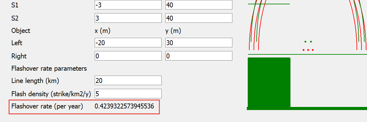
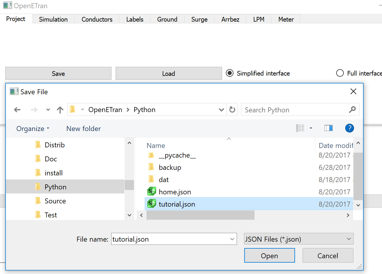
Back at the *Phase View* window, we can use the critical currents to calculation line flashover rate. Click the *Flashover Rate* button, and then navigate to your critical current file, as shown below.

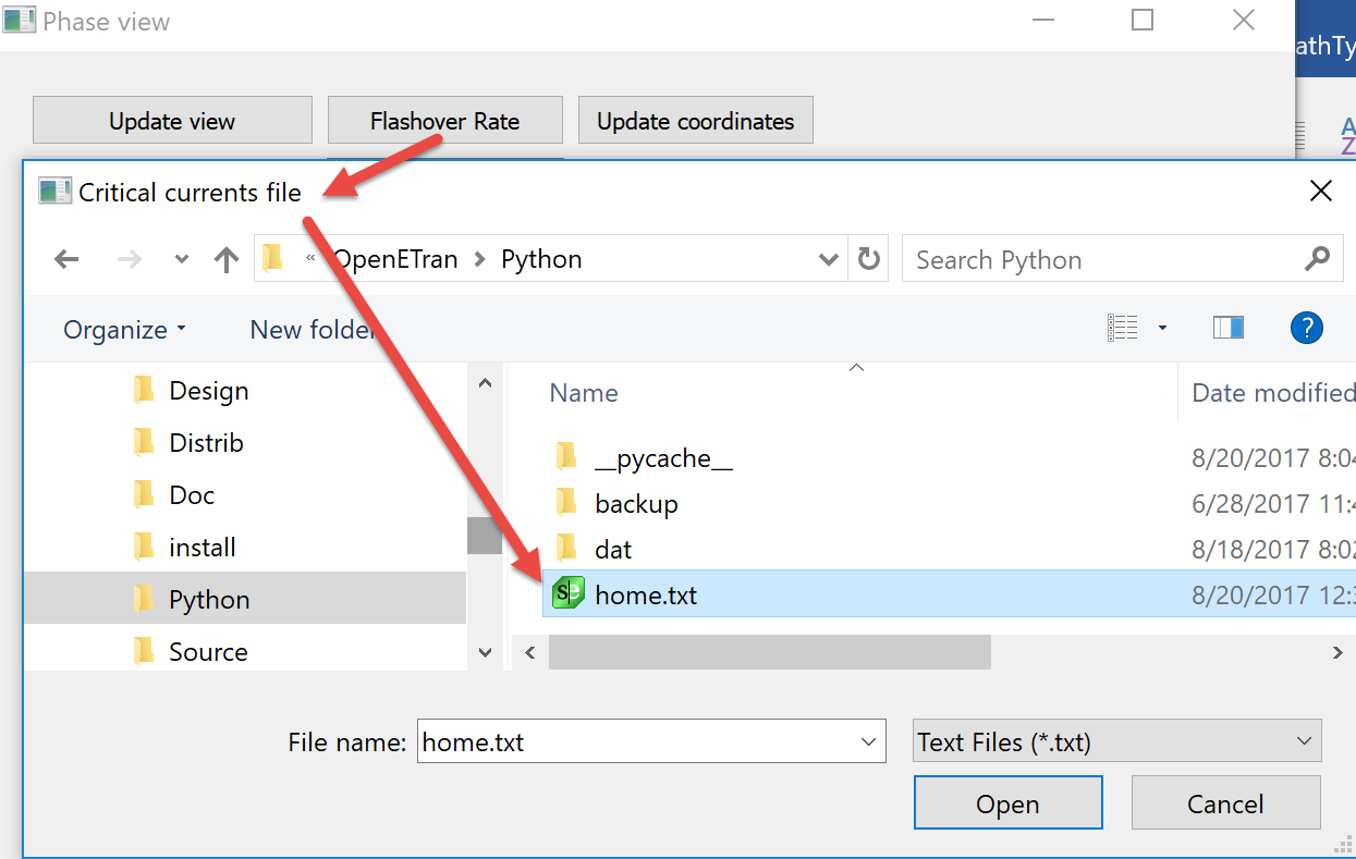
Click *Open* in the file open dialog, and then see an estimated flashover rate of 0.42 per year for the given parameters.

Save your data again, as it may be used in the next section of this tutorial.

500-kV Line Arresters

Line arresters have been used for transmission line protection more often in recent years. If actual vendor data is not available, the following table provides some typical data.

System Voltage Level [kV]	500	345	230	138	115
MCOV [kV]	318	209	160	88	76
10-kA Discharge Voltage [kV]	901	607	497	330	288
FOWPL [kV]	991	668	546	354	325
Lead Length [m]:	1.5	1.2	0.9	0.6	0.6

Building on the previous section, we can explore the benefits of line arresters for the 500-kV line. If necessary, re-load the 500-kV line data from the last section, using the “Load” button:

Run the critical current simulation, and verify that you get the same results as before:

In beta, it’s necessary to re-enter the critical current simulation setup and the flashover rate setup from the previous section.

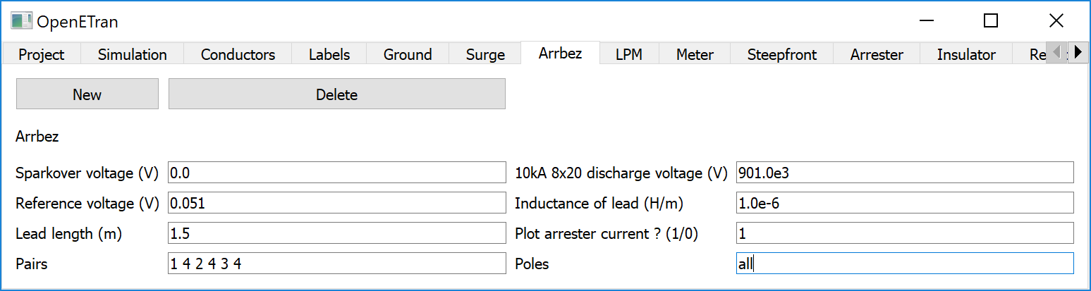
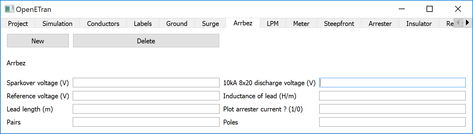
On the Arrbez tab, enter typical data as follows for a line arrester from phase to ground on every tower:

If you then re-run the one-shot simulation, two plots appear, one for all the arrester currents and one for the struck tower voltages. The voltage waveshapes look similar to the ones from before, but the peak insulator voltage magnitudes are reduced slightly, from 865 kV to 781 kV. These values were already below the CFO and the arrester 10-kA discharge voltage.

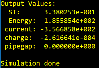
In the console window, there are three non-zero arrester outputs for total energy [J], peak current [A] and total charge [C] for the most-stressed arrester in the model. These can be used for evaluating arrester duty; see the newer IEC arrester standards for more information.

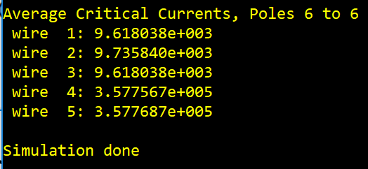
Run the critical current simulation again, and see that the critical current values for strokes to all 5 conductors have increased (note: 500 kA is the maximum critical current that OpenETran will use, so in this case, the critical current for strokes to the shield wire is practically infinite).

The flashover rate performance does not finish in Python.

It may be more interesting to replace the counterpoise with ground rods, and see if the lightning performance is still acceptable with just line arresters. On the Ground tab, change the data to 100-Ohm ground rods, and **blank out** the counterpoise data:

Now run the critical current simulation again, and see the results are only slightly higher than with counterpoise: Flashover calculation hangs.

To see what happens with 100-Ohm grounds and no line arresters, **blank out** the Arrbez data:

Run the critical current simulation again. The critical current for strokes to the shield wires are only 36 kA, so this design won’t perform very well. Flashover calculation hangs.

15-kV Distribution Line: CFO Added

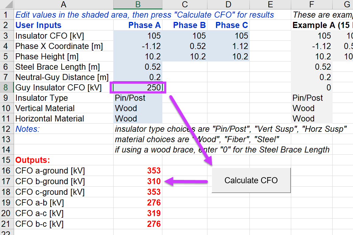
This example is based on the 15-kV distribution line described on pp. 36-37 of [2]. Without line arresters or shield wires, nearly every direct stroke to a distribution line will cause flashover. However, if the CFO is 300 kV or more, flashovers from nearby strokes will be practically eliminated. To achieve this level of insulation strength, it’s important to account for CFO added by various pole materials. A CFO-added tool has been provided, for Microsoft Excel, in the file *CFO_Added.xlsm*. This tool incorporates a Visual Basic for Applications (VBA) program, so you have to “enable macros” to use it.

The spreadsheet comes pre-loaded with this example, and as seen below, the goal of 300 kV CFO is not met, especially on the middle phase.

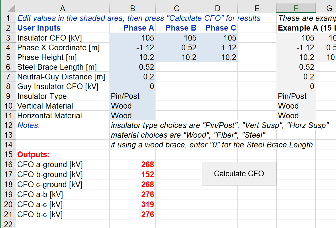
One method of increasing the CFO is to add a guy insulator, and as illustrated by the revised calculation below, the CFO is now at least 310 kV on each phase. However, two of the phase-to-phase CFO values are estimated at 276 kV. This won’t matter much for nearby strokes, as each phase has approximately the same induced voltage from nearby strokes, but it could influence results for direct strokes. OpenETran allows you to model phase-to-phase insulation, in addition to phase-to-neutral.

The spreadsheet also includes data for a 35-kV shielded distribution line, pp. 37-39 of [2], but we won’t use it here.

Following steps like in section 2, you can build this line in the Python GUI. In order of the tabs, please enter the following data:

This line has 50-Ohm grounds at every other pole, with all phase-neutral and phase-phase CFO values as estimated with the CFO-added method. If you run the one-shot simulation, the voltage plots indicate several insulator flashovers, even for 10-kA stroke current. When the Python console shows a severity index (SI) of 1.0, it means at least one insulator flashed over. Some of the plotted voltages reach peak values above the CFO, but then flashover early in the simulation according to the time-dependent leader progression model (LPM). At the CFO, flashover would occur at around 15 microseconds, but in this case, flashovers occur at around 1.5 microseconds.

In the critical current setup, we need to strike a pole with ground (#5) and one without (#6), but we don’t need to strike the neutral (#4) because the phase wires are above it.

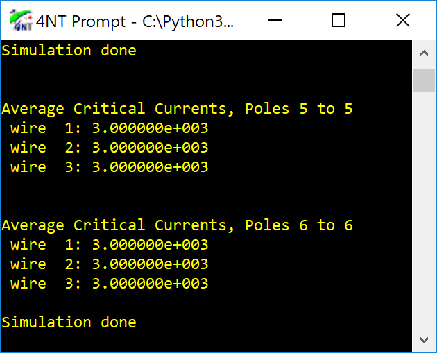
Running the simulation, we see that the critical currents are 3 kA (OpenETran’s minimum) at both poles and all three struck wires, because we haven’t really provided any lightning protection. Every stroke to the line will cause flashover.

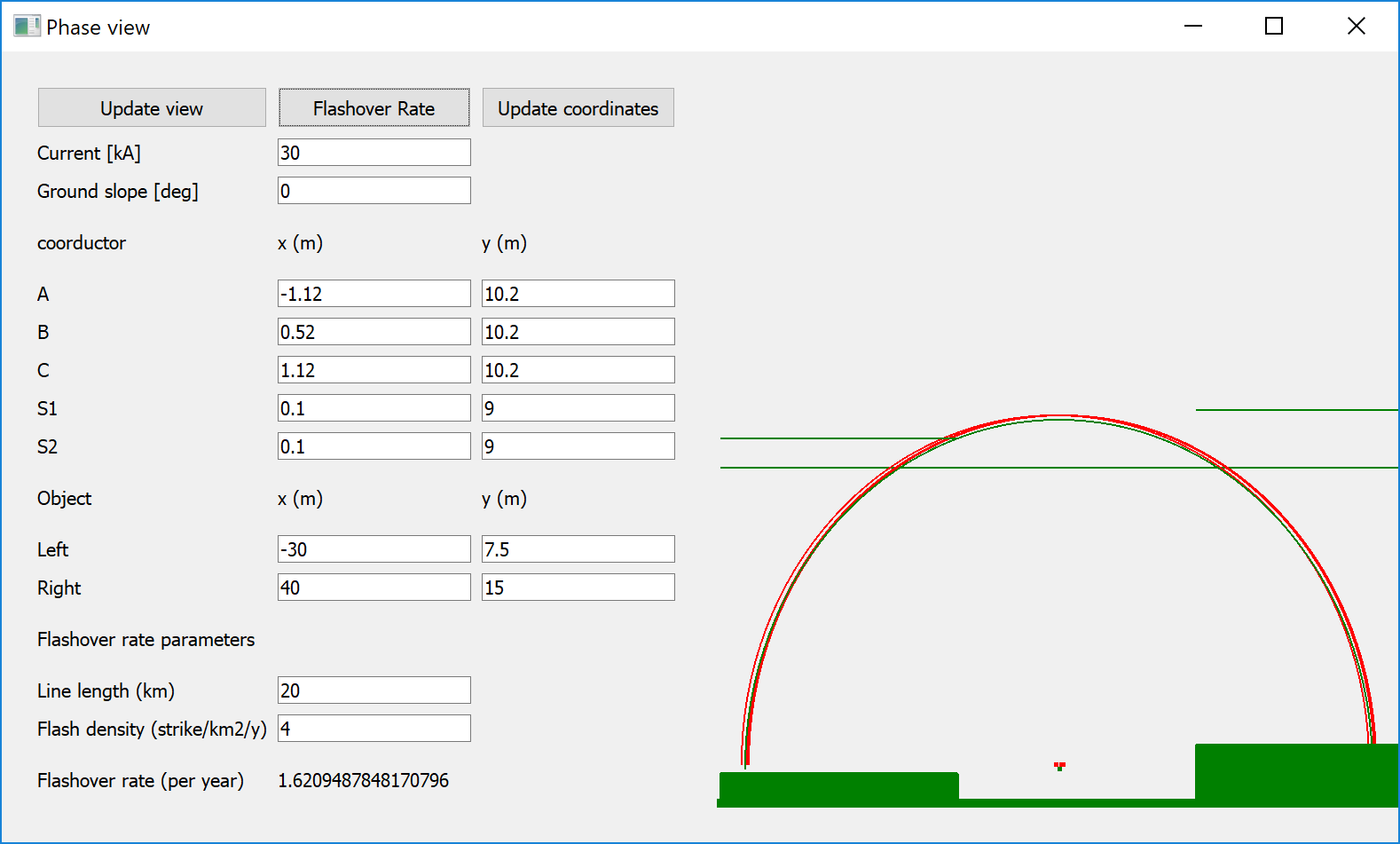
Over in the Phase View window, click “Update coordinates” and then enter data as shown below. As the project only contains 4 conductors, you should manually set the S2 coordinates equal to those for S1. This view represents a row of houses on the left of the line, and a row of trees on the right. At 30 kA, these nearby objects do partially shield the line. When you click “Flashover Rate” and load the file of 3-kA critical currents, the flashover rate is 1.62 per year. If you zero out the nearby Object data, and repeat the “Flashover Rate” calculation, this result increases to 4.15 per year.

To get better performance for direct strokes, we might consider the following:

• Add line arresters to odd poles, i.e., all those having a ground in the base case.
• Ground every pole, and put line arresters on every pole.
• Add an overhead shield wire, as in Example B of [2]. Considering the low CFO values, this option might not work well without also implementing lower ground impedances and/or line arresters.

15-kV Distribution Line: Open Point Protection

This example modifies the previous one, to consider the protection of an open tie point on the distribution line. We’re going to look at pole #11, for a stroke to pole #10, which is one 50-m span away. We’ll remove all the LPM insulators in order to clearly show the transient voltages at the open point. Make changes on the following three tabs to match:

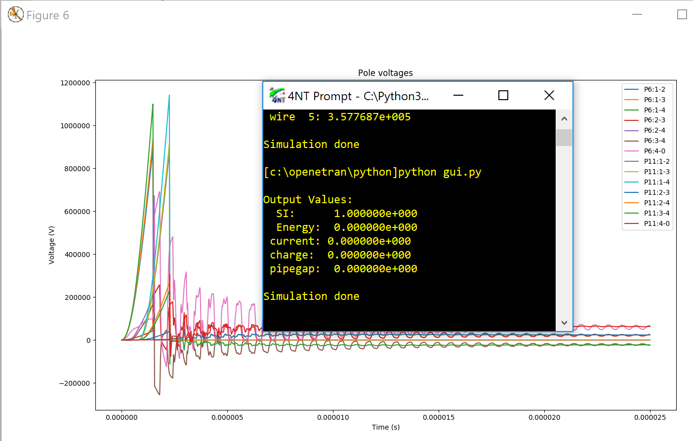
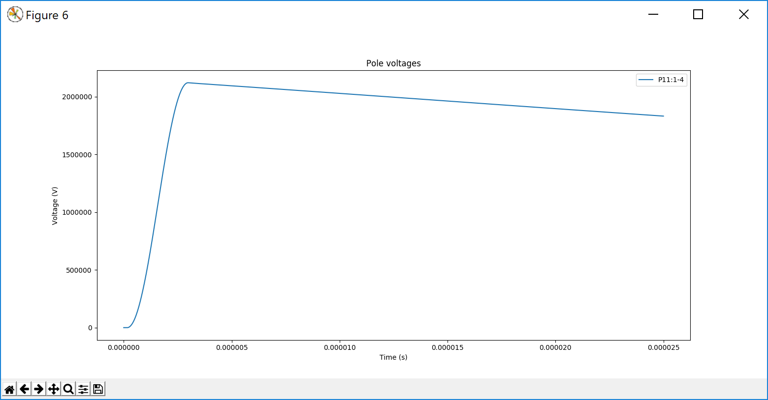
Run the one-shot simulation, and observe the monitored voltage is 2122 kV! It wouldn’t actually reach that level if we still had LPM insulators in the model.

To show the effect of an open point, change the right-hand termination from a surge impedance (1) to open (0):

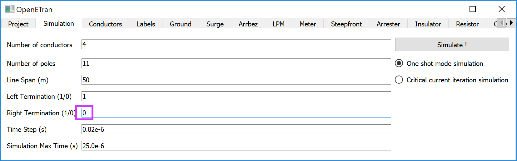
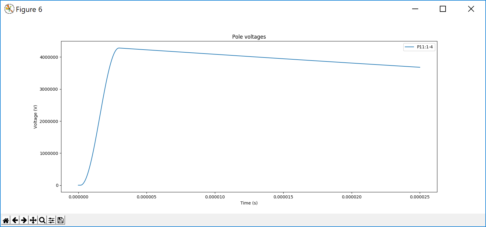
Run a one-shot simulation again; the waveshape is about the same but the peak voltage approximately doubles at the open point, as expected from traveling wave theory:

Now put an arrester just at the monitored point, as shown below.

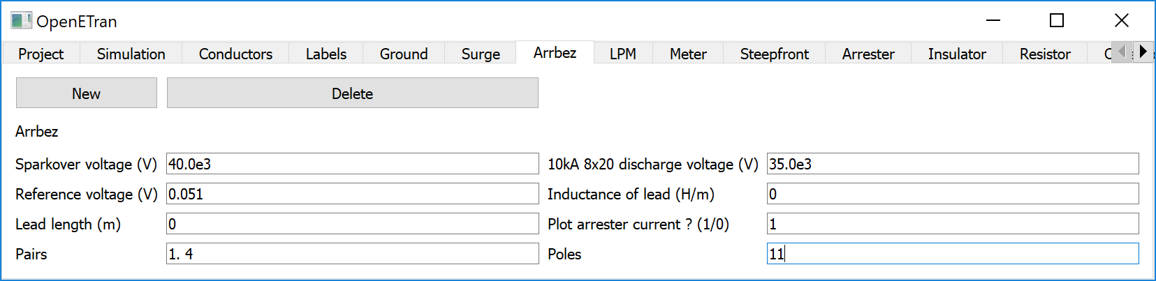
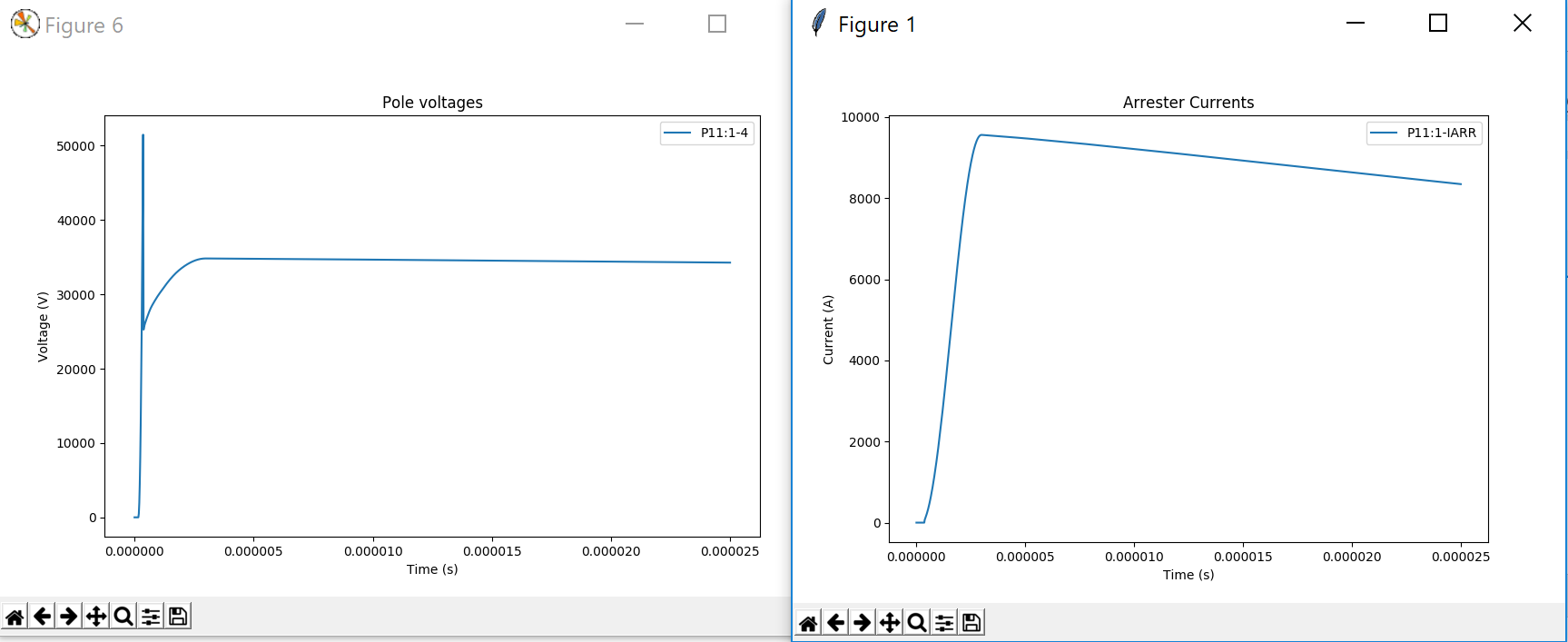
After running a one-shot simulation again, we obtain two plots for the arrester voltage and current. Nearly all of the stroke current discharges through the arrester; the rest goes to the left of the stroke point and into the left-hand surge impedance termination. The arrester peak voltage is about 51 kV, because of time-dependent conductance within the arrester, and the sparkover characteristic (not common in modern arresters, but included here for illustration). The arrester lead inductance, if modeled, would also have an effect.

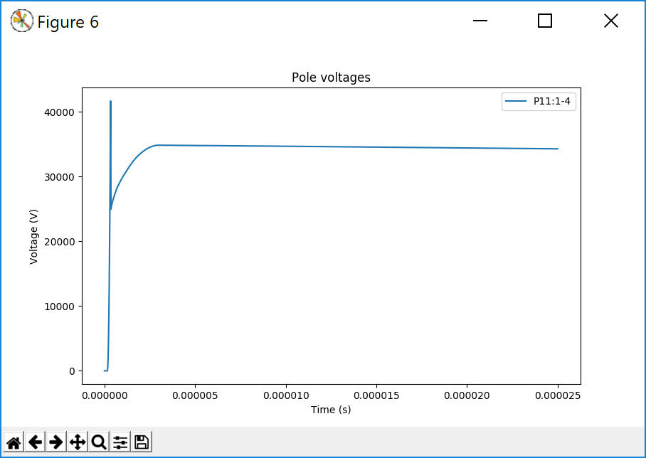
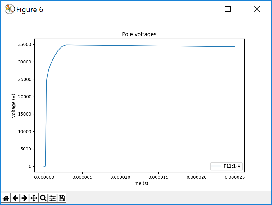
If we change the “Reference voltage” parameter from 0.051 to 0, the time-dependent conductance is disabled but we still have the sparkover at 40 kV (left, below). The peak voltage is a little above 40 kV due to time step discretization in the simulation. By further setting the sparkover voltage to 0, we see the peak arrester voltage is about 35 kV (right, below). As expected, the arrester protects the open tie point, but time-dependent and non-linear phenomena can have an impact.

Tutorial References

1. IEEE Std. 1243-1997, IEEE Guide for Improving the Lightning Performance of Transmission Lines.
2. IEEE Std. 1410-2010, IEEE Guide for Improving the Lightning Performance of Electric Power Overhead Distribution Lines.