Introduction¶

This program simulates the effect of direct lightning flashes to electric power distribution lines. The main application would be analysis of the effect of surge arresters, pole grounding, and insulation strength on the flashover rate from direct flashes to the line. A planned enhancement to the program will simulate nearby lightning flashes. Another application is the simulation of surges entering a substation from a shielding failure or backflash out on the line.

The solution algorithms are similar to those used in the “industry standard” Electromagnetic Transients program (EMTP) [1]. However, the program input and overall structure have been customized and simplified for this particular application.

Figure 1 shows the circuit structure analyzed for overhead lines. It includes a series of one or more poles, with each pole connected by a section of line with one or more conductors. One conductor, typically the neutral, may be grounded at selected poles or at all poles. Each line section must have the same span length and conductor configuration. Figure 1 also shows optional features, connected to some of the poles. These include:

Insulators
Surge arresters
Terminations, with optional D.C. voltage bias
Meters for plotted voltage output
Meters for arrester, pole ground, and service drop currents
Surge current to represent a direct flash to a conductor

The program can also simulate lumped resistors, inductors, and capacitors. However, it is not suitable for the study of switching transients. References [2-5] describe methods of simulating induced voltages from nearby lightning strokes. However, this has not been implemented in OpenETran yet.

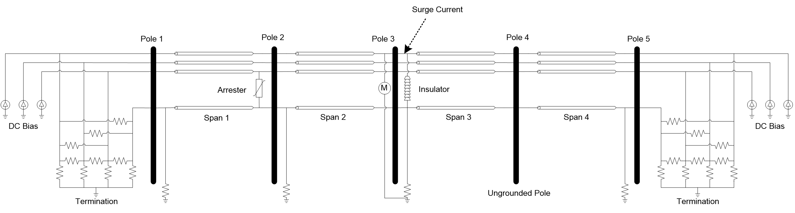
Figure 1: The circuit structure is a series of poles and line sections

Quick Start¶

Installation¶

The program is distributed as a Python package. It needs Python 3.5.3 or greater to work. In order to install it, the user first needs to download and install Python from the website www.python.org/downloads. In Python, the module needed to install packages is called “pip” and is already integrated into the Python installation in versions 3.5.3 and greater. The application “pip” is located in the “Scripts” in the Python installation folder.

If the OpenETran software is already on the user’s computer in a prebuilt “.whl” wheel format, the user needs to open the Windows command prompt and use the command “pip install PATH\OpenETran_win-1.0.0-py3-none-any.whl”, with PATH being the path of the archive on the computer. Pip will then download the dependencies and install the software automatically. An executable program, “OpenETranGUI.exe”, will be created in the Scripts folder of the Python installation. Once created, this executable is the entry point of the program. The user only needs to double click on it in order to launch the OpenETran program. It is also possible to move the application in another folder on the machine.

Tutorial¶

The tutorial section of this document includes step-by-step examples using the GUI and console mode extensions:

500-kV horizontal line from IEEE Std. 1243-1997
15-kV wooden crossarm line from IEEE Std. 1410-2010
35-kV shielded line with standoffs from IEEE Std. 1410-2010
Double-circuit transmission line from the GUI and console mode

User Interface Reference¶

The program can be run in several different modes.

Console Interface – One-Shot Mode with Plot Files¶

The program in one-shot mode reads an input file, and creates one or two files for printed output and plot data. The command to execute one-shot mode is:

Command: *OpenETran –plot elt overhead *

Reads: overhead.dat

Writes Plot Data File: overhead.elt

Writes Output File: overhead.out

Note that the program always uses file extension .dat for input files, .out for text output files, and .elt for binary plot output files. The program only creates plot data if the input file specifies voltage or current outputs. The complete plot file options include:

*plot none* to skip the creation of plot files
*plot elt* for a binary plot file with .elt extension
*plot csv* for a comma-delimited text plot file with .csv extension
*plot tab* for a tab-delimited text plot file with .txt extension

The binary voltage and current meter outputs may be plotted with The Output Processor (TOP) software. The file type to open in TOP is called “EPRI Lightning Transients” and the file extension is *.elt. See the TOP manual or on-line help for more information. The text files may be plotted in Excel, MatLab, or a variety of other programs.

Console Interface – Critical Current Iteration Mode¶

The program in critical-current mode reads an input file and creates one files for output. No plot data is created in this mode. The command to execute critical-current mode is:

Command: *OpenETran –icrit pole1 pole2 wires… overhead *

Reads: overhead.dat

Writes Output File: overhead.out

Note that the program always uses file extension .dat for input files and .out for text output files. The command-line arguments for this mode are:

*pole1* is the number of the first pole to hit, according to the numbering convention defined in the input file.
*pole2* is the number of the last pole to hit, according to the numbering convention defined in the input file. If pole1 and pole2 are not equal, the program will average the critical currents for all poles numbered pole1 through pole2, inclusive. This averaging may not be what the user would want. Therefore, it is recommended to set pole2 = pole1, run the program separately for each pole, and handle the critical current output separately from each critical-current mode run.
*wires…* are a sequence of integer flags, 0 or 1, identifying each wire (i.e. conductor) that should be considered for critical current analysis. The sequence of exposed wire flags must match the conductor sequence defined in the input file. If there are not as many flags as conductors, the remaining conductors are not included in the critical current analysis.

The output will include the critical stroke current that just causes flashover of any insulator in the model, constrained between 3 kA and 500 kA. For an example of using this mode, see the run_icrit_tests.bat and test_icrit.dat text files provided in the test sub-directory. The graphical interface described in section 3.3 also supports critical-current mode.

Graphical User Interface (GUI)¶

The OpenETran GUI is divided in two windows. One provides a conductor visualization tool for easier analysis of the phase exposure to lightning and calculation of the flashover rate. The other is a tab window that allows an easier and more productive use of OpenETran than in console mode.

Main window – OpenETran¶

Figure 2 and Figure 3 illustrate the input window of OpenETran. This is a tab window, with one tab for each type of component that can be modeled, following the input template described in section 5. Most of these components were illustrated in Figure 1. Two simulation modes are available on the simulation tab, as seen in Figure 2, and it is possible to add and remove elements dynamically using the “Add” and “Delete” buttons, as seen in Figure 3. In the “Project” tab, it is possible to write a project name and save/load it. It is also possible to switch between the full and simple interface, where the tabs “Steepfront” to “Pipegap” are hidden.

The simplified interface configuration should suffice for most line design applications. The full interface exposes little-used components. In some cases, there are two choices for modeling an item:

For line surge arresters, use *Arrbez* (simple interface) instead of *Arrester* (full interface)
For line insulators, use *LPM* (simple interface) instead of *Insulator* (full interface)
For lightning strokes, us *Surge* (simple interface) instead of *Steepfront* (full interface)

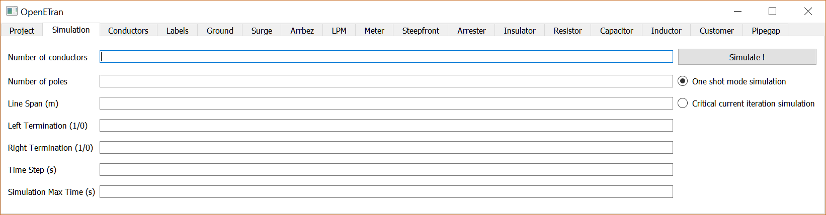
Figure 2: Simulation tab of the GUI

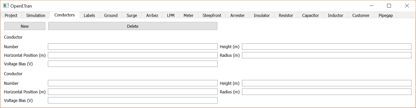
Figure 3: Conductor tab of the GUI

When in “One shot simulation mode”. Clicking the “Simulate” buttons launches OpenETran, then the GUI reads the output .csv files and displays the needed curves. An example of a displayed curve is shown in Figure 4.

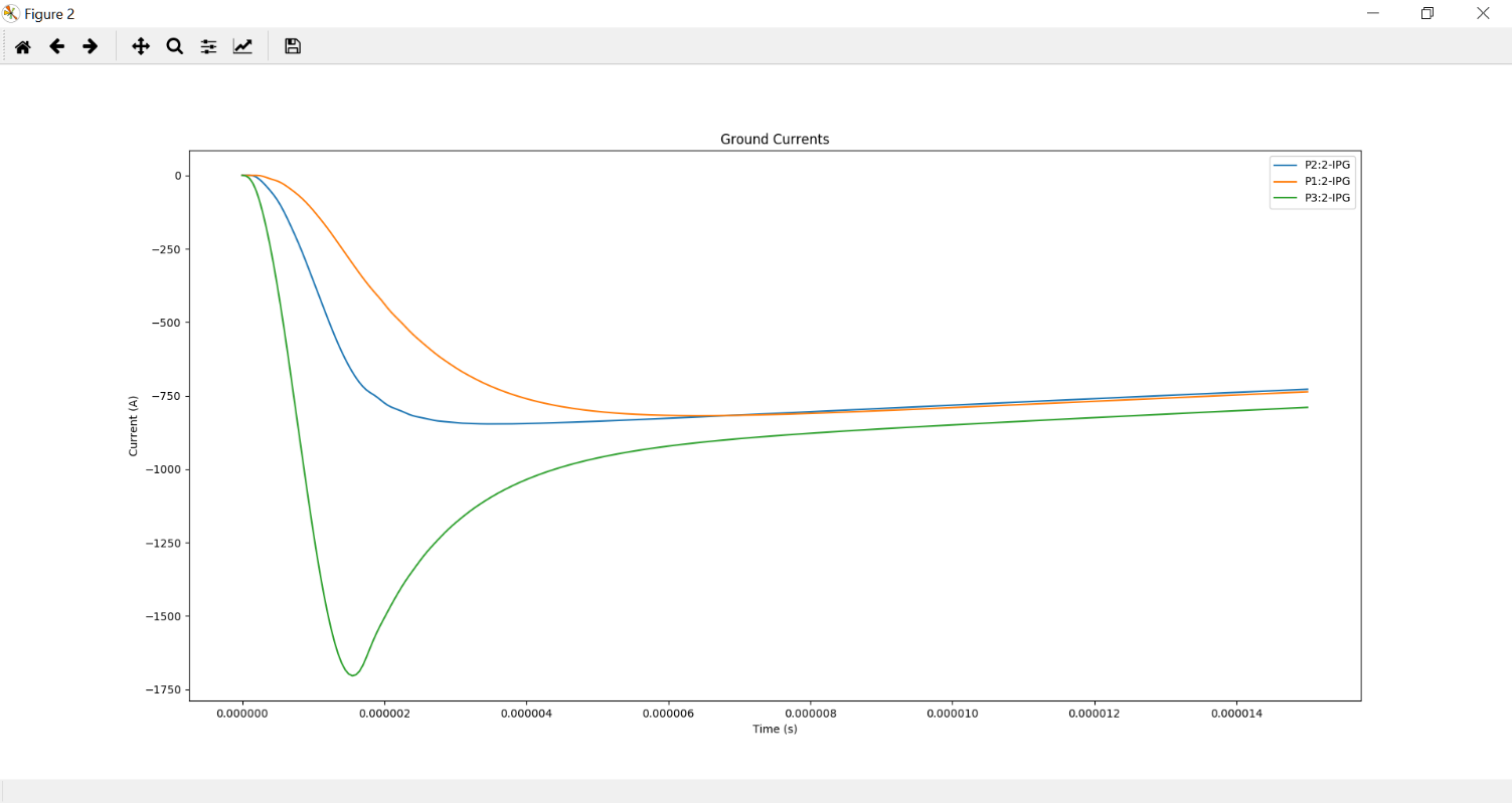
Figure 4: Ground current curves

In case of an error in OpenETran, the output is displayed on the Python console.

Finally, when simulating in critical current mode, the user needs to specify the first and last pole to hit and the wire sequence. In the wire sequence, the user defines which conductors are to be considered in the analysis. For example, in a 4-wire system, the wire sequence ‘1 0 1 1’ means that wires 1,3 and 4 are considered, wire 2 is discarded. The GUI will then call OpenETran in -icrit mode several times for each pole in the pole sequence. The critical currents are then printed in the Python console and written in a text file, in the same folder as the input file. This critical current output file is then used when calculating the flashover rate, as explained in section 3.3.2.

Secondary window – phase visualization and flashover rate calculation tool¶

The secondary window of the GUI, as seen in Figure 5, serves as a visualization aid to the user designing the system to minimize the phase exposure to direct strokes and reduce the flashover rate.

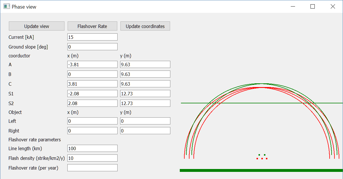
Figure 5: Visualization window of the OpenETran GUI

The red dots and red arcs are, respectively, the phase wires and phase exposure arcs determined by the critical current value. The green dots and green arcs are for the shielding wires connected to the top of the poles/towers. The lower green line represents the striking distance to ground. Two other lines, if present, determine the striking distances to nearby objects (e.g. houses, trees) on either side of the line. If the height of those nearby objects is 0, these lines coincide.

To calculate the flashover rate, the user needs to push the “Flashover Rate” button. The program then prompts the user to choose a critical current text file, that was previously generated using an OpenETran critical current simulation. The GUI then uses these critical currents, the line span between poles, the flash density, the exposure width of the line and the probability of a first stroke current to exceed the critical current from the IEEE 1243 and 1410 standards:

\[P(I > I_{\text{Crit}}) = \frac{1}{1 + \left( \frac{I_{\text{Crit}}}{31} \right)^{2.6}}\]

Since the output critical current file provides critical currents at different poles of the line, the GUI first calculates the yearly flashover rate at each pole. The displayed result in the label is the average of all these flashover values to reflect the weight of each pole on the total flashover rate on the line.

Technical Reference¶

The multi-conductor overhead line sections are subject to the following simplifying assumptions:

Earth return path has perfect conductivity.
Conductors have no resistance.

These assumptions produce the following self and mutual surge impedances for travelling waves:

\[Z_{\text{ii}} = 60\ ln\frac{2h_{i}}{r_{i}}\ \Omega\]

\[Z_{\text{ij}} = 60\ ln\frac{D_{\text{ij}}}{d_{\text{ij}}}\ \Omega\]

Where:

i, j = conductor #’s
h = conductor height [m]
r = conductor radius [m]
d = distance between two conductors [m]
D = Distance between conductor i and image (below ground) of conductor j [m]

The transmission line equations are then decoupled into single-phase modes. Because of assumption #1 above, travelling waves propagate at the speed of light in all modes. The travelling wave model is similar to EMTP’s [1].

As an alternative to conductor data, the user may input the surge impedance and travelling wave velocity directly. This option is only available for uncoupled conductors. This option is useful for cables, which have lower surge impedances and travelling wave velocities than overhead lines. It can also be used for surge arrester leads.

All other model components are connected to poles. The solution of these lumped component models is also similar to EMTP’s [1]. The following paragraphs describe model characteristics for these lumped components.

Bus conductor¶

The typical kinds of bus conductor include:

round tube, described by outside radius R0
angle, described by side lengths L and W, and wall thickness t

3. IWCB, also described by side lengths L and W, and wall thickness t

These bus conductor types are simulated by adjusting the input conductor radius. Round tubes are modeled the same way as stranded overhead line conductors. Because all high-frequency current is assumed to flow on the surface of the conductor, the round tube’s outer radius is input.

In both the angle and IWCB types, high-frequency currents tend to concentrate in the corners. Based on finite element simulations, it is apparent that currents in the angle bus concentrate on the two open edges, but not on the interior corner. Currents in the IWCB bus will concentrate on all four corners of the square or rectangle. The standard formulas for bundled conductors can approximate these distributions of current. The equivalent bus conductor radius is:

\[r_{\text{equiv}} = \sqrt[N]{\text{Nr}A^{N - 1}}\]

\[A = \frac{\sqrt{L^{2} + M^{2}}}{2}\]

Where:

N = number of conductors in bundle, 2 for angle and 4 for IWCB
r = subconductor radius = t/2
t = bus wall thickness
L = one side length of angle or IWCB cross section
W = adjacent side length of angle or IWCB cross section
A = radius of circle through subconductor centers

There will be a slight error in using these equations for IWCB with rectangular rather than square cross sections.

For example, consider the self-impedance of a single bus conductor at height 10 meters. For a round tube, the outside diameter is 6 inches, or 0.1524 meters. For the angle and IWCB, the length and width are both 0.1524 meters, and the wall thickness is 0.5 inches, or 0.0127 meters. The equivalent radii and surge impedances are shown in Table 1.

Table 1: Bus conductor surge impedances

Bus Type	N	r	A	r_equiv	Z
Round Tube	1	0.0762	N/A	0.0762	334.2
Angle	2	0.00635	0.1078	0.0370	377.6
IWCB	4	0.00635	0.1078	0.0751	335.1

The IWCB has nearly the same surge impedance as a round tube with similar outer dimensions, while the angle bus has higher surge impedance. There will be no effect on mutual surge impedances between bus conductors.

Surge Current¶

There are two surge current waveshape models in the program. The *surge* component uses a 1-cosine front. This component was used in EPRI’s LPDW version 1.0 through 4.0, including the transmission line simulations in version 4.0. A *steepfront* component, with concave front, was added for EPRI’s SDWorkstation.

1-cosine Front¶

The surge current waveshape has a 1-cosine front, and an exponential tail decay. As Figure 3 shows, this waveshape has a “toe” at the front and a relatively flat peak. For a direct flash to the line, a surge current should be connected from the struck conductor to ground. The program allows a delayed starting time for the surge, which would shift the waveshape in Figure 6 to the right.

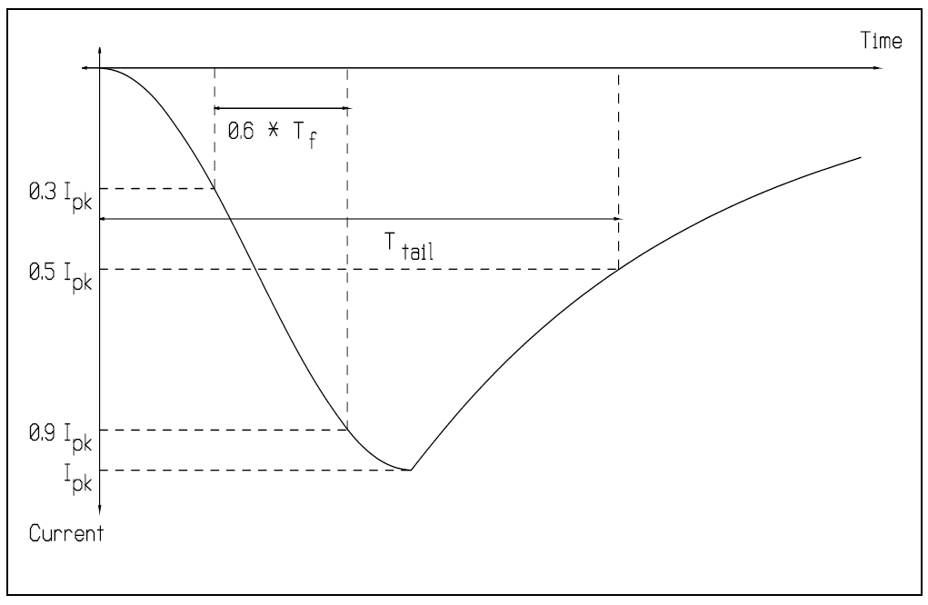
Figure 6: 1-cosine Surge Current Parameters

Concave Front¶

Typical lightning current surges have a pronounced toe, flat peak, and maximum current steepness near the peak of the surge. Based on [13], the *steepfront* surge component uses Bezier splines to define a current front with maximum steepness at 90% of the crest value, with a flat peak and exponential tail. In contrast, the 1-cosine shape has maximum steepness at 50% of the crest value. Figure 7 shows a 30-kA surge, with 3.67-us front, represented by the two different surge models. The concave shape reaches its peak later, but its virtual zero based on the 30% and 90% points also occurs later. This difference in virtual zeros must be accounted for when constructing volt-time curves for insulators. Both shapes have the same front time, based on the 30% and 90% points. The concave shape is more realistic, and could produce higher voltages in arrester-protected systems, due to the higher maximum steepness.

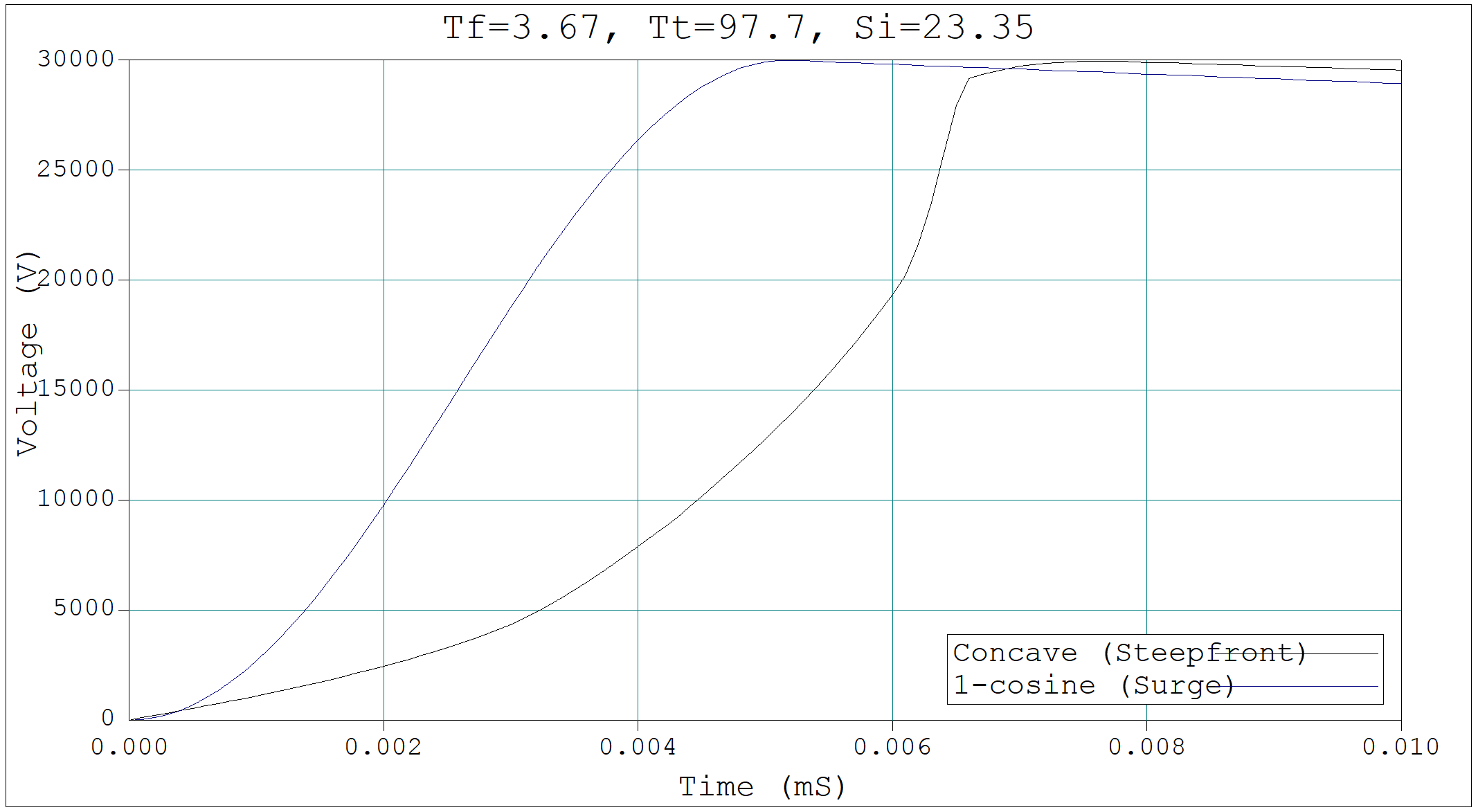
Figure 7: Typical Lightning Surge Current Parameters, surge vs. steepfront Models

Insulators¶

Insulators may be connected between pairs of conductors, or between a conductor and ground. The typical phase insulator would be connected from a phase conductor to the neutral conductor, rather than from phase conductor to ground. There are two insulator models available. LPDW version 1.0 through 4.0 used the destructive effect model, while SDWorkstation and later versions of DFlash used the leader progression model.

Destructive Effect Model¶

The program integrates voltage across the insulator to determine a “Destructive Effect”:

\[DE = \int_{}^{}{\left( e - V_{b}^{\beta} \right)\text{dt}}\]

With:

e = Magnitude of voltage across insulator
V_b = minimum breakdown voltage
β = exponent

When the DE exceeds a critical level, then the insulator flashes over. This equation simulates the volt-time curve, as illustrated in Figure 8. For an insulator with Critical Flashover Voltage of 100 kV, typical parameters are:

V_b = 0.0
β = 5.42434
DE_max = 8.4265 E+21

The program integrates DE only when the magnitude of “e” exceeds Vb. The program maintains both positive and negative polarity DE values, either of which may produce a flashover. If the voltage changes polarity, the DE value is maintained until the voltage changes polarity again. Thus, the DE values can never decrease during a simulation; they may only increase or remain constant. This crudely simulates the leader progression process.

Each insulator is an open circuit, not affecting the simulation, unless the destructive effect across the insulator exceeds the critical level. At that instant, the insulator becomes a short circuit, connecting the two conductors for the rest of the simulation.

If the insulator does not flash over, the program outputs a “per-unit severity index.” The insulator would probably flash over if the voltage across the insulator were increased by a factor 1.0/SI, but kept the same waveshape.

Leader Progression Model¶

The leader progression model is based on the based on the physics of flashover [13], whereas the destructive effect method is more of a curve-fitting approach. The leader progression model generally gives more accurate results.

Only the leader propagation time is modeled; the corona inception time and streamer propagation time are ignored. The program keeps track of the remaining unbridged gap length in both positive and negative directions. The leader propagation velocity is:

\[\frac{\text{dx}}{\text{dt}} = Ke(t)\left\lbrack \frac{e(t)}{x} - E_{0} \right\rbrack\]

Where:

K = propagation constant
E0 = breakdown gradient
x = unbridged gap length
e(t) = voltage across gap

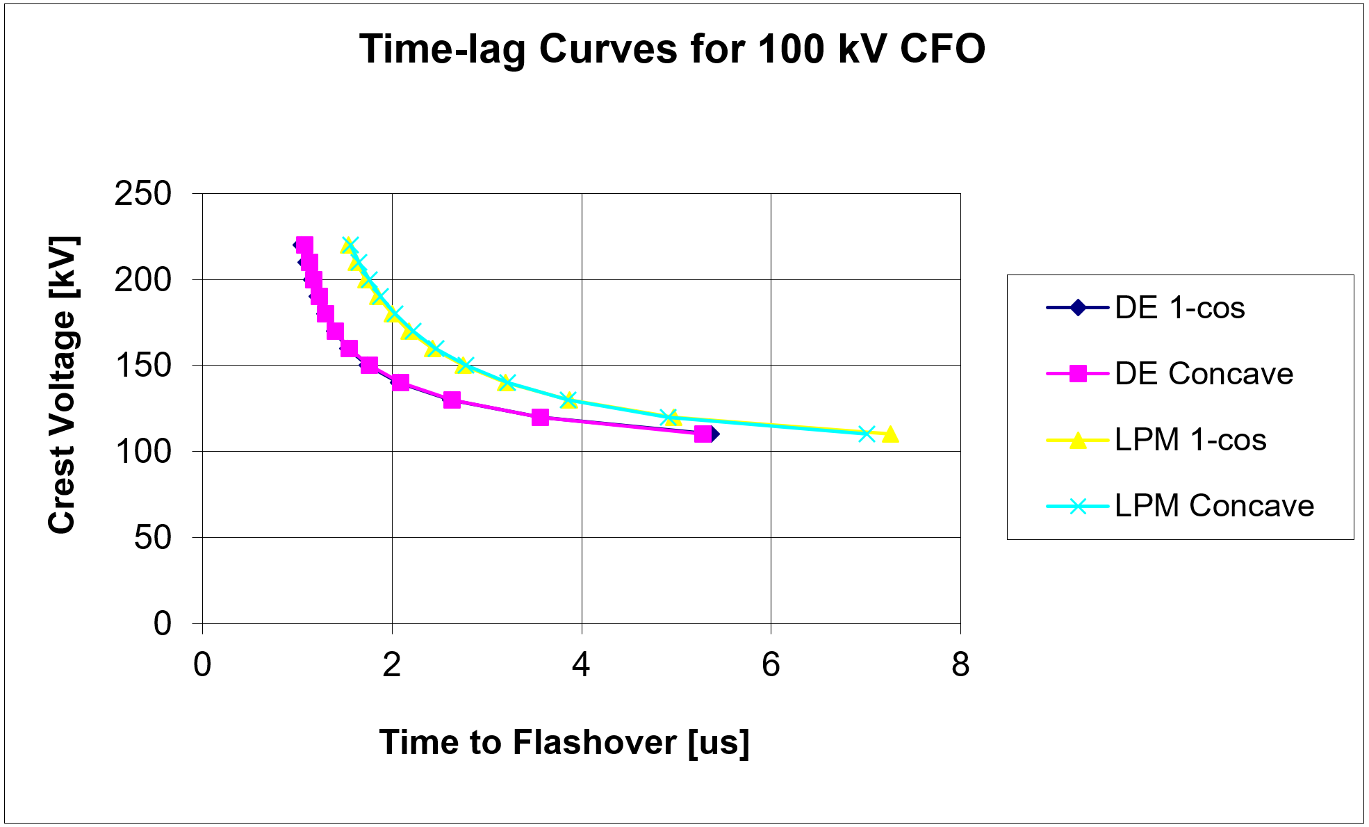
Figure 8: Air-Porcelain Insulator Volt-Time Curves, Destructive Effect and Leader Progression Models

The unbridged gap length, x, starts at a value given by CFO / E0. Two instances of this equation are integrated at each time step, one for positive e(t) and one for negative e(t). Only one leader can grow at each time step, and only if e(t) exceeds E0.

For air-porcelain insulations, E0 = 535.0e3 and K = 7.785e-7. For apparatus insulations, E0 = 551.3e3 and K = 1.831e-6.

Whenever either the positive or negative leader’s x reaches zero, the insulator flashes over. The program can also run in a mode where insulator flashovers are disabled. The waveshape across each insulator is saved in memory. At the end of the simulation, the saved waveshape is scaled up and down using the bisection method to determine the crest voltage that just barely causes flashover. This produces the severity index for each insulator. The severity index can be greater than one if insulator flashovers were disabled. If an insulator flashover occurs during the simulation, the output severity index is 1.0.

Figure 8 shows the volt-time curves for a 100 kV CFO insulation in air, using both insulator models. Each model was run with both 1-cosine and concave surge waveshapes for a 1.2 x 50 waveshape, but Figure 8 shows that the surge front model had little impact on the results. Figure 8 shows that the leader progression model takes longer to flash over at a given crest voltage.

At voltages below the CFO, Figure 9 shows that flashovers can still occur with the destructive effect model, which might be considered a defect. These flashovers can be eliminated by using a non-zero value for Vb, but then the curve fit isn’t as good at higher voltages and lower flashover times. The leader progression model should work better over a wider range of crest voltages and times to flashover.

Figure 9: Volt-Time Curves Extended to Long Flashover Times

Surge Arresters¶

There are two surge arrester models available. Both models have optional built-in series gap and lead inductance. LPDW versions 1.0 through 4.0 used a simple switched model, with one linear segment for the discharge characteristic.

If the surge arrester gap sparks over, it will conduct until the voltage falls below Vknee. At that point, the gap recovers its full strength for voltage transients of positive or negative polarity.

The arrester model includes a built-in lead inductance, which may be input as zero. With a non-zero inductance, the output voltage at the arrester lead terminals will be increased for short impulses. However, the program keeps track of the actual arrester voltage for energy calculations.

On distribution lines, most surge arresters would be connected from a phase conductor to the neutral conductor.

Switch Model¶

A surge arrester includes a non-linear resistance designed to limit transient overvoltages. Some surge arresters have a gap that allows a higher peak transient voltage than the discharge voltage across the non-linear resistance. These characteristics are shown in Figure 10. In this program, the surge arrester switch model is an open circuit until the voltage exceeds V_gap or V_knee, whichever is greater. At that time, the discharge characteristic follows a single linear segment. Using this model, it is possible to fit two points on the discharge characteristic; LPDW versions 1.0 through 4.0 matched the 10-kA and 20-kA points.

Figure 10: Surge Arrester Switch Model

Spline Model¶

There are two built-in 8x20 discharge characteristics, obtained from the data General Electric provides for its metal oxide arresters. Both characteristics are provided in per-unit of the 10-kA discharge voltage. One characteristic is for arresters rated 48 kV and below, or a 10-kA discharge voltage of 140 kV and below. The other characteristic is for arresters rated 54 kV and above. Both characteristics are shown in Table 2; the program selects one based on the input 10-kA discharge voltage.

Table 2: Built-in Surge Arrester Discharge Characteristics

I[A]	V/V:sub:`10`
	V:sub:`10` < 140e+03 \| V:sub:`10` ≥ 140e+03
0.00	0.000	0.000
0.01	0.500	0.500
1.0	0.663	0.691
10.0	0.696	0.725
100.0	0.743	0.769
500.0	0.794	0.819
1,000.0	0.824	0.847
2,000.0	0.863	0.881
5,000.0	0.937	0.946
10,000.0	1.000	1.000
15,000.0	1.069	1.061
20,000.0	1.123	1.109
40,000.0	1.288	1.251

Figure 11 shows the simulated arrester discharge characteristics for a 1.2 x 50 current discharge of 20 kA peak through both the switch and Bezier spline models. The 10-kA discharge voltage was input as 40 kV in both cases, but the spline model is more accurate over the whole range of currents. The Bezier spline technique ensures continuous first derivatives at the breakpoints given in Table 2, with no oscillatory behavior between the breakpoints. However, the discharge voltages aren’t exactly matched at the breakpoints. The error could be made arbitrarily small by choosing more tightly spaced breakpoints.

The simulation was repeated with a piecewise linear model. Figure 12 shows the region around the characteristic’s knee, and the Bezier spline’s error at the breakpoints is not significant.

For steep wavefronts, the surge arrester inductance plus lead inductance adds to the discharge voltage, primarily near the peak of the discharge current because the dI/dt is highest near the peak. Test results show that the discharge voltage peaks well in advance of the discharge current peak. This effect cannot be represented with just a series inductance.

The Cigre method [14] adds a turn-on conductance in series with the inductance and nonlinear discharge characteristic. The conductance starts at zero, and increases with time according to:

\[\frac{\text{dG}}{\text{dt}} = \frac{G_{\text{Ref}}}{T}\left( 1 + \frac{G}{G_{\text{Ref}}} \right)\left( 1 + \frac{G}{G_{\text{Ref}}}\left( \frac{I}{I_{\text{Ref}}} \right)^{2} \right)\exp\left( \frac{U}{U_{\text{Ref}}} \right)\]

G₀ = 0

T = 80

\[G_{\text{Ref}} = \frac{34}{U_{10}}\]

I_Ref = 5.4

U_Ref = kU₁₀

Where: U₁₀ = 10-kA discharge voltage, in kV

U = voltage across the arrester, in kV

I = current through the arrester, in kA

k = constant ranging from 0.03 to 0.05, depending on manufacturer

The effect is to delay the start of current conduction through the arrester, while the voltage continues to build up. Figure 13 shows a discharge characteristic with turn-on conductance, and with series inductance plus turn-on conductance. The upper part of the loop tracks the front of the wave, and the lower part of the loop tracks the tail. With just the turn-on conductance, the discharge voltage is increased only in the range from 0 to 5 kA on the wave front. This is caused by an effective delay in the start of conduction. With both turn-on conductance and series inductance, the discharge voltage is increased all the way up to the 20 kA peak on the wave front.

An IEEE working group has presented another model for these dynamics [15], using two nonlinear resistors, along with some linear resistors and inductors. The IEEE model can be implemented with off-the-shelf EMTP components, but requires iterative parameter adjustments to tune the model for each arrester. The Cigre model proved more convenient for this program, because the series inductance and time-dependent turn-on conductance could be built into the arrester model.

Figure 11: Arrester vs. Arrbez Model, 20kA, 1x20 Discharge Current

Figure 12: Bezier Spline vs. Piecewise linear Characteristic, 20kA, 1x20 Discharge Current

Figure 13: Arrbez Turn-On Conductance and Inductance Model, Uref = 0.051, L = 0.3 μH, 20 kA, 1x20 Discharge Current

Pole Grounds¶

Single ground rod model¶

The neutral conductor at each pole, or at selected poles, is grounded through a resistance. The impulse ground resistance is less than the measured or calculated 60-Hz resistance, because significant ground currents cause voltage gradients sufficient to break down the soil around the ground rod. The following equations govern this behavior:

\[I_{\text{brk}} = \frac{\rho E_{0}}{2\pi R_{60}^{2}}\]

\[R_{\text{Ground}} = \frac{R_{60}}{\sqrt{1 + \frac{I_{\text{Ground}}}{I_{\text{Brk}}}}}\]

Where: E₀ = soil breakdown gradient, typically 400 kV/m

ρ = soil resistivity [Ω-m]

R₆₀ = measured or calculated 60-Hz ground resistance [Ω]

These equations assume that the pole ground consists of a single ground rod, which is typical of distribution lines. The program uses a supplemental current injection to model the decreasing resistance. The ground model includes a built-in pole downlead inductance, which may be input as zero. With a non-zero inductance, the output “ground” voltage will increase for steep current fronts. The model does not include capacitance in the pole ground.

Counterpoise model¶

The user can also choose to add a counterpoise (grounding wire) to the model. The counterpoise is modeled like a transmission line with distributed parameters, as seen in Figure 14.

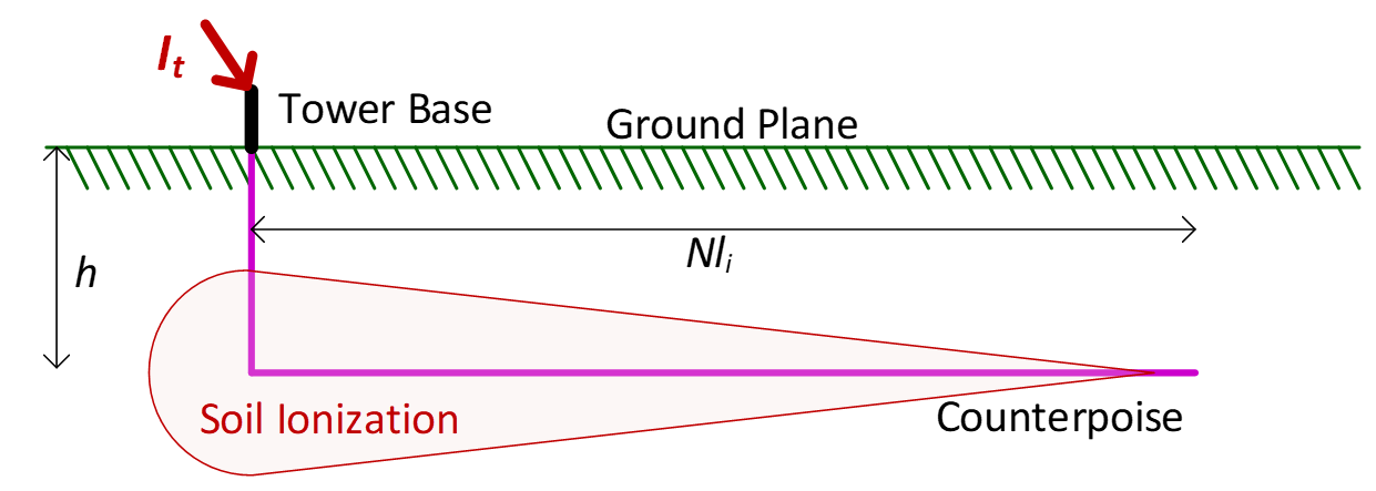
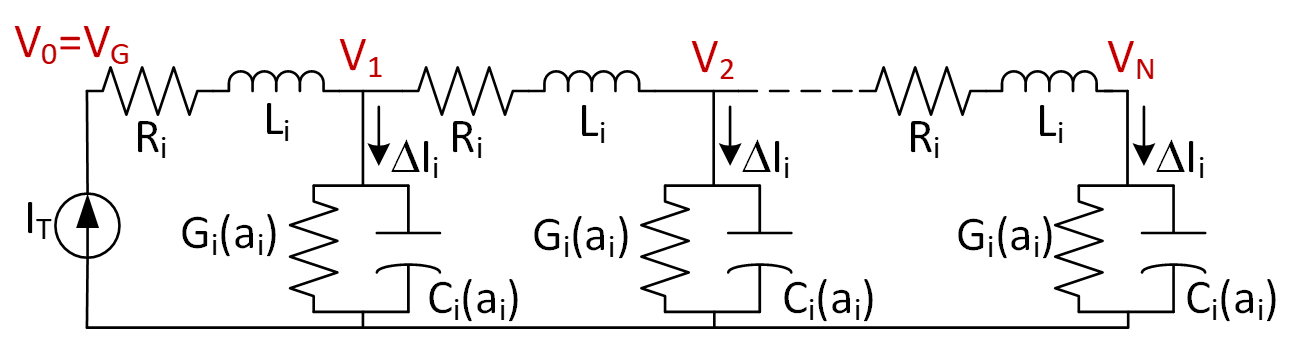
Figure 14: Representation of a ground electrode with nonuniformly lumped parameters

The model operates as described in [6] and modified in [7]. Additional input parameters are:

l = total length of the counterpoise [m]

a = radius of the counterpoise [m]

h = depth of the counterpoise [m]

ε = relative ground electric permittivity

ρ = ground resistivity [Ω/m]

n = number of segments; a typical value is 20

As current leaks into the ground through shunt G and C elements, the soil ionizes and the effective radius, a, increases. In turn, this changes the G and C values in each segment. Overall, the counterpoise model is nonlinear and changes at each time step of the simulation.

Power Frequency Source¶

The program can automatically add a surge impedance termination at each end pole in Figure 1. This termination absorbs travelling waves, with no reflections back into the circuit model. The program calculates this termination to match the input conductor data. The program can also run with either or both end poles left open-circuited.

The program can also simulate a power frequency bias voltage on one or more conductors. The bias is modeled as a D.C. voltage, assuming the power frequency voltage will not change very much during the short time of interest for lightning transients.

Initial conditions for the line sections, plus any capacitors and inductors, are calculated to support this D.C. bias voltage. Injected currents are added to each end pole termination, to maintain the bias voltage across each surge impedance termination.

The bias voltage is input with the conductor data. First, convert the nominal line-to-line RMS voltage to peak volts line-to-ground. Then, select a phase A voltage angle. The conductor bias voltages for a 13.8- kV system, with instantaneous phase A voltage angle of 20 degrees, would be:

\[V_{\text{peak}} = 13,800 \bullet \frac{\sqrt{2}}{\sqrt{3}} = 11,268\ V\]

\[V_{A} = 11,268 \bullet \sin\left( 20 \right) = 3,854\ V\]

\[V_{B} = 11,268 \bullet \sin\left( 20 + 240 \right) = - 11,097\ V\]

\[V_{C} = 11,268 \bullet \sin\left( 20 + 120 \right) = 7,243\ V\]

\[V_{N} = 0\]

Because the bias voltage is D.C., any lumped inductors connected between phase conductors must include some series resistance. A pure inductance cannot support a D.C. voltage (V = L dI/dt = 0 for D.C.). Even with a series resistance, the solution for an inductor with D.C. bias would probably not be valid for the actual situation with an A.C. “bias.” Lumped inductors should not be used in this program with a power frequency bias, unless the inductor is connected from neutral to ground (and the neutral has no power frequency voltage).

Pole-Top Transformer and Service Drop¶

The program can simulate the house ground current and transformer secondary terminal X2 current, according to a simplified model [8]. Normally, the transformer would be attached to a pole with a primary arrester and a pole ground. The program automatically adds a house ground with service drop inductance, and connects it to the pole.

Assuming the house load is shorted by gap sparkover in the service entrance meter, the X2 terminal current is:

\[I_{X2}\left( t \right) = k_{1}I_{\text{hg}}\left( t \right) + k_{2}\int_{}^{}{V_{P}\left( t \right)\text{dt}}\]

Where: I_hg = simulated house ground current

V_P = simulated primary transformer voltage

k1 and k2 are constant coefficients that depend on the transformer and service drop inductances [8]. k2 is zero if the transformer secondary winding inductances are balanced. k1 is much less for triplex service drops than for open-wire service drops. k1 increases somewhat if the transformer has interlaced secondary windings, which have lower inductances than non-interlaced windings.

Pre-discharge currents¶

Pre-discharge currents flow between two parallel conductors, or a pipe gap, when the voltage between them exceeds the insulation breakdown voltage [12]. Pre-discharge limits the voltage and delays final breakdown by a few microseconds or more. The effect can be modeled as a simple surge arrester connected between the conductors, with a knee voltage equal to the Critical Flashover Voltage (CFO), and a single slope resistance of 4300 ohm-feet, or 1311 ohm-meters. The resistance is lower, and more current flows, between longer conductors.

Pre-discharge currents only begin to flow when the voltage exceeds the pipe gap’s CFO. It is possible to coordinate the pipe gap to protect substation equipment insulation. On an overhead line, however, the pole or tower insulation is the weak link, because its CFO is less than the CFO of the air gap between the conductors (which governs the flow of pre-discharge current). Figure 15 illustrates this coordination problem for a single-phase distribution line. Using an air breakdown gradient of 610 kV/m (186 kV/ft), the CFO between conductors is estimated at 744 kV. At the pole, the pin insulator and wood combine for an estimated CFO of 328 kV. The “protective level” provided by the pipe gap is over twice the CFO of the insulation to be protected.

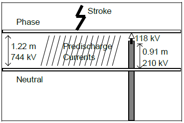
Figure 15: Pre-discharge Currents on a Signe-phase Line

Generally, the main effect of pre-discharge currents is to make midspan flashovers much less likely. Instead, flashovers occur at the pole. The PIPEGAPS.DAT, PAPERGAP.DAT, and PAPERARR.DAT test cases illustrate the use of this model. The OpenETran.exe screen output labeled “pipegaps” is the largest pre-discharge current through any of the line sections, in amps. Usually, this line section with maximum pre-discharge will be next to the stroke location.

Critical current iterations¶

Critical currents are determined for each requested pole and conductor, using the GSL Brent-Dekker root-finding method [16] on this function:

\[F\left( I \right) = \text{SI}_{\max} - 1 + (T_{\max} - t_{\text{flashover}}) \bullet 10^{5}\]

I is the simulated peak stroke current. SImax is the maximum severity index over all insulators in the model, which equals one if a flashover occurred. Tmax is the requested simulation time and tflashover is the actual simulation stopping time; this is less than Tmax if a flashover occurred. The function F(I) is negative if no flashover occurs, and it decreases in magnitude as insulators come closer to flashover. When a flashover occurs at exactly Tmax, the function F(I) is zero, which is the desired root. When the flashover occurs more quickly, F(I) becomes more positive. This monotonic and smooth behavior of F(I) allows the root-finder to determine the critical current within 0.01 kA, usually within 10 iterations.

Based on [13], the critical current iterations are done with a fixed front time of 3.83 s. The tail time (to half value) is fixed at 103.638 s. For an exponential tail, this produces the median first-stroke charge of 4.65 C at the median first-stroke peak current of 31.1 kA.

Striking distances to phases and ground¶

In the visualization tool, as explained in section 3.3.2, the user can see clearly the vulnerability zones of the conductors in the line along with the striking distance to ground. The striking distance to a conductor r_C and to ground r_G are defined in IEEE Std. 1243 as:

\[r_{C} = 10I^{0.65}\]

\[r_{G} = \frac{\beta r_{C}}{\cos\alpha}\]

Here, I is the current going through the conductor and α is the ground slope, which can be between 0 and 45 degrees in the software. The term β is defined as:

\[\begin{split}\beta = \left\{ \begin{matrix} 0.37 + 0.17 \bullet \log_{10}\left( 43 - h_{\max} \right),\ \ if\ h_{\max} < 43m \\ 0.55\ ,\ \ \ \ \ \ \ \ \ \ \ \ \ \ \ \ \ \ \ \ \ \ \ \ \ \ \ \ \ \ \ \ \ \ \ \ \ \ \ \ \ \ \ \ \ \ \ \ \ \ \ \ \ \ \ \ \ \ \ if\ h_{\max} > 43m \\ \end{matrix} \right.\\end{split}\]

With h:sub:`max` defined as the height of the highest conductor in the system.

Input and Output Formats¶

The program input format for an overhead line is shown in Table 3. DFlash used this type of format. CFlash and SDW used an alternate form of input for network models, described in Section 5.7. The input must be created with a text editor and saved in a file before running the program. Note that when using the Python GUI, the user does not need to fill the input file, it is done automatically.

The program uses SI (metric) units for input:

meters
seconds
volts
amperes
ohms
ohm-meters
henries
farads
volts per meter

Exponential notation may be used for numerical input:

1.0e-6 for 1 ms
-10.0e3 for -10 kA

Floating point input data may have a decimal point. Inputs that are defined as integers must not have a decimal point.

Text input may be upper or lower case, or a mixture, but the spelling of keywords must be correct. All model parameters must be provided in the correct order, and no missing parameters are allowed.

Inputs on the same line must be separated by one or more blanks or tabs. There may be any number of blank lines between the data entries in Table 3.

Comment lines begin with an asterisk (*).

Table 3: Transients Program Input Formats for Non-Network System

N_Cond	N_Pole	Span	l_term	r_term	dT	Tmax	(required)

Conductor	#	h	x	r	Vbias	[Sag]	[Nb]	[Sb] (Ncond entries
Conductor	#	h	x	r	Vbias	[Sag]	[Nb]	[Sb] required)

ground	(-)R60	r	E0	L	d	(required)
	h	lt	n	eps		(opt.)
pairs	…
poles	…

surge	I_peak	T_front	T_tail	T_start
pairs	…
poles	…

steepfront	I_peak	T_front	T_tail	T_start	S_I
pairs	…
poles	…

arrester	(-)V:sub:gap	V_knee	R_slope	L	d
pairs	…
poles	…

arrbez	V_gap	V₁₀	U_Ref	L	d	amps
pairs	…
poles	…

insulator	CFO	Vb	β	DE
pairs	…
poles	…

lpm	(-)CFO	E0	K_L
pairs	…
poles	…

meter	type
pairs	…
poles	…

labelphase	N	C

labelpole	N	P

resistor	R
pairs	…
poles	…

inductor	R	L
pairs	…
poles	…

capacitor	C
pairs	…
poles	…

customer	R_hg	r	E₀	L_hg	d	N	L_p
	L_S1	L_S2	L_cm	r_A	r_N	D_AN	D_AA
	L
pairs	…
poles	…

pipegap	V	R
pairs	…
poles	…

*Notes for Table 3:*

pairs … = one or more pairs of conductor #’s for component connections, at the specified poles.

conductor 0 = ground

limits: 0 < conductor # < Ncond

poles… = one or more pole #’s to connect components between specified conductor pairs.

“poles all” means every pole

“poles even” means all even-numbered poles

“poles odd” means all odd-numbered poles

limits: 1 < pole # < Npole

Negative R60 or Vgap requests plotted current output for grounds and arresters, respectively.

Use “Meter” components to request plotted voltage or current output. Type = 0 (or blank) for voltage, 1 for arrester/arrbez current, 2 for pole ground current, 3 for customer house ground current, 4 for transformer X2 terminal current, 5 for pipegap current.

The “Customer” component produces plotted house ground and X2 terminal currents automatically.

For plotted arrester and pole ground current output, input the first numerical parameter with a negative sign (-Vgap for arresters, -R60 for grounds). For plotted arrbez currents, set “amps” to 1.

Negative CFO for the lpm component disables insulator flashover during simulation, but severity index is calculated at the end.

Negative V10 for the arrbez component causes piecewise linear rather than Bezier spline fit to VI characteristic.

The input file is divided into three subsections:

Required simulation control parameters
Required conductor or cable data
Optional pole component data

Required Simulation Control Parameters¶

These five parameters must be input on the first non-blank line in the file, in this order:

Ncond (integer): number of conductors. A three-phase line with neutral would have Ncond = 4.
Npole (integer): number of poles in the circuit. The poles are numbered from 1 to Npole.
Span (float): line section span length in meters. For distribution lines, the span length is probably between 20 and 100 meters.
lt (integer): 1 to terminate pole at left end, 0 to leave open
rt (integer): 1 to terminate pole at right end, 0 to leave open
dT (float): simulation time step in seconds. As a rule of thumb, choose dT as the smallest of the following two values:
1. dT = 0.1 * Tfront (for a surge input)
2. dT = 0.2e-6 * (span / 300.0)
Tmax (float): maximum simulation time in seconds. Tmax should be at least three times Tfront for the surge current input. To calculate surge arrester discharge duties, Tmax should be at least two times Ttail for the surge current input.

Required Conductor Data¶

There must be one line for each conductor. The conductors are numbered in sequence from 1 to Ncond. In addition, conductor 0 is “remote ground.”

Each line of conductor data begins with the “conductor” keyword, followed by data in the following order:

# (integer): conductor number, from 1 to Ncond
h (float): conductor height above ground, in meters. Use the height at the pole, or an average height accounting for sag.
x (float): conductor horizontal position, in meters. Use the pole centerline as a reference, and enter conductors to “left” of the centerline with negative x, conductors to the “right” with a positive X.
r (float): conductor radius, in meters.
Vbias (float): instantaneous power frequency voltage, in volts to ground. See the previous section for equations to calculate Vbias. Enter 0.0 for conductors with no power frequency voltage.
Sag (float): mid-span sag, in meters. This is optional; defaults to 0.
Nb (integer): number of sub-conductors in a bundle. This is optional; defaults to 1.
Sb (float): bundle sub-conductor separation, in meters. Must be input > 0 if Nb > 1.

The last “conductor” may be a pole node, with no physical conductor attached. This is entered in the form “node #”. A typical usage is for arrester-protected lines with no grounded conductor. All arresters and phase-ground insulators are connected from phase to the pole node, and then the pole ground is connected from the pole node to 0.

A sample conductor configuration is shown in Figure 16.

Instead of the preceding “conductor” input, the alternative “cable” keyword may be used, followed by this data:

# (integer): conductor number, must = 1
Z (float): surge impedance [Ohms]
V (float): travelling wave velocity, in meters per second
Vbias (float): instantaneous power frequency voltage, in volts to ground

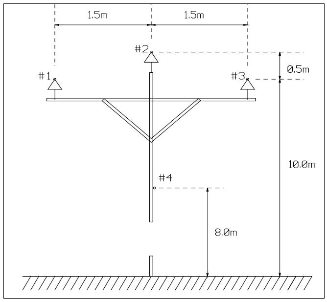
Figure 16: Example Conductor Configuration

Optional Pole Components¶

Input for lumped components connected to poles must follow the required conductor data. Each section of optional input contains three lines, with no intervening blank lines, as follows:

Identifying keyword and component parameters
Conductor pair connection
Pole locations

These optional sections may be placed in any order in the input. A useful simulation case would include at least a “surge” input, but the program does not require this. An input file with no optional components would produce constant output voltages equal to the conductor bias voltages. Also, there would be no voltage output without some “meter” components.

There may be more than one input section for each type of optional component. For example, there might be two separate “insulator” components for the phase-to-ground and phase-to-phase insulation. There might also be two separate “arrester” components with identical characteristics, but one requests plotted currents at a selected pole, while the second places arresters at other poles and requests no plotted current output.

The optional component keywords and parameters follow:

ground parameters: R60: measured or calculated low current ground resistance in Ohm (if R60 is < 0, the ground current will be output for plotting)

ρ: soil resistivity in Ω-m (typical ρ = 250Ω-m)

E:sub:`0`: soil breakdown gradient, in V/m (typical E₀ = 400kV/m)

L: inductance per unit length of downlead

d: length of downlead in m (may be 0)

h: depth of counterpoise in m (optional)

lt: total length of counterpoise in m (optional)

n: number of segments for the counterpoise (optional)

eps: relative permittivity of ground (optional)
surge parameters: I:sub:`peak`: crest current, in amps

T:sub:`front`: 30-90 front time, in seconds

T:sub:`tail`: 50% fail time, in seconds

T:sub:`start`: surge starting time after simulation time 0, in seconds (usually 0)
steepfront parameters: I:sub:`peak`: crest current, in amps

T:sub:`front`: 30-90 front time, in seconds

T:sub:`tail`: 50% fail time, in seconds

T:sub:`start`: surge starting time after simulation time 0, in seconds (usually 0)

S:sub:`I`: maximum current steepness, in per unit of 30-90 steepness
arrester parameters: V:sub:`gap`: sparkover voltage for arresters that have gaps, in V

V:sub:`10`: 10-kA, 8x20 crest discharge voltage from manufacturer’s catalog, in volts. Negative V10 signifies piecewise linear characteristic, rather than Bezier spline fit.

U:sub:`Ref`: reference voltage for dynamic turn-on conductance, in per-unit of V10

L: inductance per unit length of arrester lead

d: arrester lead length in consistent units (may be 0.0)

amps: use 1 to plot arrester current, 0 otherwise
insulator parameters: CFO: critical flashover voltage, in volts

(usually 95.0e3 < CFO < 500.0e3 for phase-to-neutral insulators)

Vb: minimum voltage for destructive effect calculation at 100 kV CFO

β: exponent for destructive effect calculation

DE: minimum destructive effect to cause flashover when the CFO is 100 kV
lpm parameters: CFO: critical flashover voltage, or BIL, in volts. A negative number indicates these insulators will not flashover during simulation, but severity index will be calculated at the end. SDW runs in this mode. E0: minimum breakdown gradient, in V/m. Use 535.0e3 for air-porcelain insulations, and 551.3e3 for apparatus insulations. KL: Use 7.85e-7 for air-porcelain insulations, and 1.831e-6 for apparatus insulations.
meter parameters: type: 0 (or blank) for voltmeter

1 for arrester or arrbez current

2 for pole ground current

3 for customer house ground current

4 for customer transformer X2 terminal current

5 for pipegap discharge current
labelphase parameters: N: wire number, from 0 to Ncond

C: character label for plots in TOP (eg., G, N, A, B, C)
labelpole parameters: N: pole number, from 0 to Npole. For network input, N must correspond to one of the poles input with line data.

name: location label for plots in TOP (eg., xfmr). No embedded blanks are allowed. For 16-bit versions of TOP, it is best to limit “name” to 5 characters.
resistor parameters: R: resistance, in Ω
inductor parameters: R: series resistance, in Ω

L: series inductance, in henries
capacitor parameters: C: capacitance, in farads
customer parameters: Rhg: 60-Hz house ground resistance, in Ω

ρ: soil resistivity, in Ω-m

E:sub:`0`: soil breakdown gradient, in volts per meter

Lhg: inductance per unit length of house ground downlead, in henries per meter

d: house ground lead length, in meters

N: transformer turns ratio

Lp: transformer primary winding inductance, in henries

LS1, LS2: secondary winding inductances, in henries
pipegap parameters: V: the CFO between conductors, in volts

(If V is < 0, the pipegap current will be output for plotting.)

R: series resistance to pre-discharge currents, in Ω

Each optional component parameter line must be followed by two lines for “pairs” and “poles.” These lines specify where the components are connected. Each component will have identical parameters. During the simulation, the program will track the status of individual grounds, insulators, arresters, and other components at each location.

“Pairs” input¶

The keyword “pairs” is followed by pairs of integer conductor numbers specifying the component connections at each pole. Conductor #0 is ground. For example:

pairs 4 0 specifies connection from conductor 4 (neutral to conductor 0 (ground)

pairs 1 4 2 4 3 4 specifies three component connections, from conductors 1, 2, and 3 to 4

For a “customer” component, the second conductor in the pair will have the house ground attached. This should be the neutral conductor.

“Poles” input¶

The keyword “poles” is followed by one or more integer pole numbers. The program also recognizes short-cuts “all”, “even”, and “odd” in place of the integer pole numbers. The specified poles and pairs are used to place components in the circuit model.

The following example places a ground (without counterpoise) at each odd-numbered pole, from conductor 4 to ground. The pole downlead has a 5-μH inductance:

ground 85.0 250.0 400.0e3 0.5e-6 10.0

pairs 4 0

poles odd

The following example places a surge only at pole 16, from conductor 1 to ground:

surge -10.0e3 1.0e-6 50.0e-6 0.0e-6

pairs 1 0

poles 16

Program Output¶

Certain portions of the input produce output, as shown in Table 4. This output will appear on screen or in a file, according to the program execution commands described in the next section.

For meter, insulator, and arrester output, the individual components are identified by pole number and the conductor pair numbers.

The Output Processor (TOP) software may be used for plotting voltage and current waveforms from binary plot files.

Network system input¶

Normally, the first line of text input specifies the number of poles and conductors. The program lays the poles out in series, and each span has the same length and conductor configuration.

An alternate form of input can be used for other topologies, including a substation network or feeder laterals. In this case, the first line of text input specifies the maximum number of conductors used in any span. In the next section of input more than one conductor geometry can be specified. Each of these input geometries will define a span type. These span types are referenced in a section of line inputs, in which poles are explicitly created as needed at the end of each line.

When using the network option, the first non-comment, non-blank text input line must be of the form:

“time” Ncond dT Tmax

*time* is a keyword, and the other three parameters are similar to those defined in Section 5.1

Following the time control card, one or more span definitions are input. These are similar to the conductor and cable inputs described in Section 5.2, with an additional span identifier before each span definition:

“span” Span_id

*span* is a keyword, and Span_id must be a unique integer. Whenever conductor geometry is input for a span definition, there can be no missing conductors. There must be Ncond lines of conductor input for the span definition, just as in Section 5.2. But when cable impedances are input, missing conductors are allowed. If the number of cable conductors for a span definition is less than Ncond, the span definition must be terminated with “end” on a single line of input. If Ncond cable conductors appear in the span definition, do not use the “end” terminator.

A single line of input with “end” terminates all span definitions.

Following the span definitions, one or more lines are input.

“line” From To Span_id Length Term_Left Term_Right

*line* is a keyword. *From* and *To* are integer pole numbers, which the program creates if they don’t exist yet. The pole numbers do not have to be consecutive. *Span_id* refers to the conductor geometry or cable impedances entered previously. Note that the *Span_id* determines which phases are present in this line, and any power frequency offset voltage. If *Term_Left* or *Term_Right* are 1, a surge impedance termination is added at the From or To pole, respectively.

A single line of input with “end” terminates all line definitions.

Following the line definitions, any of the optional pole components may be input as described in Sections 5.3 through 5.5. Only those poles created in the line definitions may be used for these components. Some of these poles may have “missing phases”, if they are fed by spans that have less than Ncond cable conductors. These “missing phases” are solidly grounded in the simulation; they have no impact on the results because the cable conductors are uncoupled in this program.

See Table 6 and Table 7 for examples of network model input.

Table 4: Text Output

*Input*	*Output Generated*

Required Parameters	T_max and the current simulation time appear on the screen as a solution progress monitor.

Conductor Data	Surge Impedance Matrix, Z_p Modal Surge Impedances, Z_m^[1] Modal Transformation Matrix, T_I^[1]

Termination Flags	D.C. Bias Voltages, with Currents injected into surge impedance terminations
Meter	Peak voltage recorded Plot data file (voltage)
Insulator	If insulator flashes over: Time of flashover If insulator does not flash over: Per-unit severity index
Arrester	If arrester operates: Time of sparkover or turn-on Time of peak discharge current Peak discharge current [Amperes] Energy discharged [Joules] Charge discharged [Coulombs] If V_gap input < 0: Peak current recorded Plot data file (current)
Ground	If R₆₀ input < 0: Peak current recorded Plot data file (current)
Customer	Peak I_hg and I_x2 Plot data file (I:sub:hg and I_x2)
Pipegap	Peak pre-discharge current If V input < 0: Plot data file (current)
“Black Box” Values	Highest per-unit severity index of any insulator Highest energy dissipated by any surge arrester Highest current discharged by any surge arrester Highest charge through any surge arrester Highest pre-discharge current through any pipegap

Examples¶

The software distribution includes over two dozen example text input files for execution from the command line, and four test cases for execution from the spreadsheet interface.

Console Mode Examples¶

The text input files are located in a “test” subdirectory of the OpenETran installation. All except “test_icrit.dat” may be executed from the “runtests.bat ” file. Each test case run this way produces a text output file and a binary output file.

The “run_icrit_tests.bat” script runs the “test_icrit.dat” file three times. The first run determines critical current for a stroke to pole without an arrester, producing an answer of 54.15 kA. The second run determines critical current for a stroke to pole with an arrester, producing an answer of 500 kA. The third run creates a plot file for a stroke approximately equal to the critical current on a pole without arrester.

The text input files include:

ABCIGLD discharge test for Bezier spline arrester with turn-on conductance and lead inductance
ABCIGRE discharge test for Bezier spline arrester with turn-on conductance
ABEZGAP discharge test for Bezier spline arrester with series gap
ABEZLEAD discharge test for Bezier spline arrester with lead inductance
ABGAPLD discharge test for Bezier spline arrester with series gap and inductance
ARRBEZ discharge test for Bezier spline arrester model
ARRESTER discharge test for arrester switch model
ARRLEAD discharge test for arrester switch model with lead inductance
ARRLIN discharge test for piecewise linear arrester model
COUNTERPOISE test for the counterpoise in high-resistivity soil
DESTEEP destructive effect insulator model, 100 kV CFO, concave surge front
DESURGE destructive effect insulator model, 100 kV CFO, 1-cosine surge front
DRIVENLT sample run file from LPDW; three-wire line with top-phase arrester
EPRI138 incoming surge for the 138-kV substation example from the EPRI ICWorkstation training course (see Figure 18 and Table 7)
EPRI500 incoming surge for the 500-kV substation example from the EPRI ICWorkstation training course
GROUNDROD test based on COUNTERPOISE, but with a single ground rod instead
HOUSE single-phase overhead with transformer secondary model
LPMSTEEP leader progression insulator model, 100 kV CFO, concave surge front
LPMSURGE leader progression insulator model, 100 kV CFO, 1-cosine surge front
NO_FLASH leader progression insulator model, 100 kV CFO, flashover disabled and severity index greater than one
OVERBEZ 4-conductor overhead line with Bezier spline arresters
OVERHEAD 4-conductor overhead line with arrester switch models (see Figure 1 and Table 5)
PAPERARR add arresters and insulators to a three-phase line
PAPERGAP three-phase line with predischarge currents
PIPEGAPS single-phase lateral with predischarge currents
RISER single-phase cable with riser pole arrester
SAGBUNDLE based on OVERHEAD, but with sag and bundling
SCOUT 4-conductor line with arresters feeding a single-phase cable with open-point arrester (see Figure 17 and Table 6)
SPANTEST testing span/line input options with a single-phase cable terminated in surge impedance
STEEP typical first-stroke current parameters, concave surge front
SURGE typical first-stroke current parameters, 1-cosine surge front
TEST_ICRIT overhead line with arresters every other pole, for testing critical current iterations

Table 5 shows the input data for a circuit similar to that shown in Figure 1. The time step of 0.02 s was chosen to provide five steps for each line section. This also provides plenty of steps for the surge front.

The Tmax of 5 s is sufficient to determine the peak voltages at poles closest to the lightning flash. It is not sufficient to determine the energy discharged in any surge arresters that operate; that would require Tmax = 200 s or more.

Figure 16 shows the conductor configuration for this example. Conductors 1, 2, and 3 represent phases A, B, and C. Conductor 4 is the neutral. The number of poles might be increased if an insulator flashover occurs in the simulation, but 11 is recommended as a starting number. Other parameters in Table 3 were chosen to be typical of a 13.8-kV distribution line.

Table 6 shows example input for analysis of the scout arrester application, based on the circuit in Figure 12. The voltage at node 6 is of particular interest. With arresters at nodes 2 and 4, the peak voltages at nodes 6 and 7 are about the same. If the arresters at nodes 2 and 4 are removed, the peak voltage at node 6 is higher than the peak voltage at node 7.

Table 7 shows example input for a substation network model, illustrated in Figure 18. The EPRI ICWorkstation training manual discussed this example in detail. The severity index for this incoming surge is about 0.35 at all points, generally matching the results obtained by EMTP simulation in the OS/2 version of EPRI’s ICWorkstation.

Table 5: Example Program Input for Overhead Line

4	31	30.0	1	1	0.02e-06	5e-06
conductor	1	10	-1.5	0.00715	3854
conductor	2	10.5	0	0.00715	-11097
conductor	3	10	1.5	0.00715	7243
conductor	4	8	0	0.00715	0

labelphase	0	G
labelphase	1	A
labelphase	2	B
labelphase	3	C
labelphase	4	N

ground	85	250	400e3	0.5e-6	10
pairs	4 0
poles	all

arrester	42.4e3	36.8e3	0.28	1e-6	0
pairs	1 4	2 4	3 4
poles	odd

insulator	300e3	0	5.42434	8.4265e21
pairs	1 4	2 4	3 4
poles	16

meter
pairs	1 4	2 4	3 4	4 0
poles	16	17

surge	-10e3	1e-6	100e-6	0
pairs	1 0
poles	16

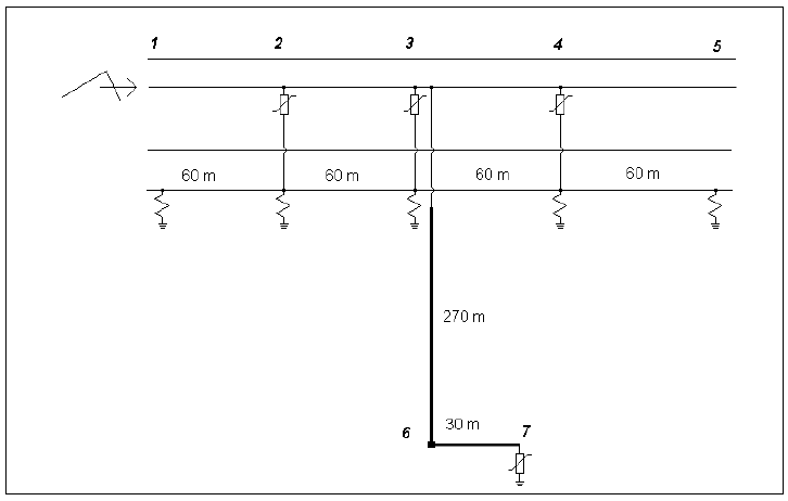
Figure 17: Scout and Cable Arrester Application

Table 6: Example Program Input for Scout Arrester Scheme

time	4	0.01e-6	15e-6
overhead line geometry
span	1
conductor	1	10	-1.5	0.00715	3854
conductor	2	10.5	0	0.00715	-11097
conductor	3	10	1.5	0.00715	7243
conductor	4	8	0	0.00715	0
single-phase underground attached to upper phase
span	2
cable	2	30	1.5e8	-11097
end
end
overhead line spans
line	1	2	1	60	1	0
line	2	3	1	60	0	0
line	3	4	1	60	0	0
line	4	5	1	60	0	1
underground spans
line	3	6	2	270	0	0
line	6	7	2	30	0	0
end

labelphase	0	G
labelphase	1	A
labelphase	2	B
labelphase	3	C
labelphase	4	N

labelpole	3	riser
labelpole	6	xfmr
labelpole	7	opntie

ground	85	250	400e3	0.5e-6	10
pairs	4 0
poles	1	2	3	4	5
riser pole, scout, and open tie arresters
arrbez	0	40e3	0	0	0
pairs	2 0
poles	2	3	4	7

surge	-10e3	1e-6	50e-6	0
pairs	2 0
poles	1

meter
pairs	2 0
poles	3	6	7

Table 7: Example Program Input for 138kV Substation

incoming backflash for the EPRI 138kV training example
time \| 1		6e-9	10e-6

network definition
span	1
cable	1	472	3.0e8	-93.0e3
end

line	1	2	10.67	0	0
line	2	3	15.24	0	0
line	2	4	9.14	0	0
line	2	5	9.14	0	0
line	5	7	9.14	0	0
line	7	8	9.14	0	0
line	6	7	10.67	1	0
line	7	9	15.24	0	0
end

labelphase	0	G
labelphase	1	A

labelpole	1	lnl
labelpole	2	cbl
labelpole	3	xfl
labelpole	4	top
labelpole	5	tiebrk
labelpole	6	ln2
labelpole	7	cb2
labelpole	8	bot
labelpole	9	xf2

meter
pairs	1 0
poles	1

source equivalent
resistor	472
pairs	1 0
poles	1

steepfront	2.54e3	1.82e-6	9.7e-6	1.0e-7	1.0
pairs	1 0
poles	1

transformers and arresters
capacitor	2e-9
pairs	1 0
poles	3	9

arrbez	0	296e3	0.051	1.57e-6	1.83	1
pairs	1 0
poles	3	9

insulators
lpm	650e3	535e3	7.785e-7
pairs	1 0
poles	all

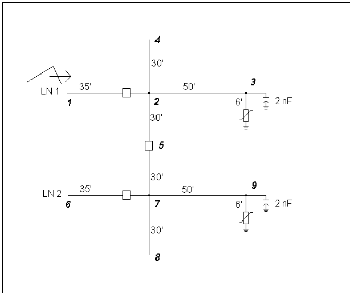
Figure 18: 138kV Substation Application

Spreadsheet examples¶

The OpenETran.xlsm file contains four examples on separate sheets. Visual Basic for Applications (VBA) macros must be enabled. In order to run each example, copy-and-paste-special the values from the example sheet onto the Input sheet. Delete any unused values from the Input sheet before clicking the Run button. Please make sure the Input data is lined up as in , and take care not to delete any named ranges from the Input sheet.

The example sheets include:

Test – four-wire line with neutral and arresters every other pole. This example should give similar results to the test_icrit.dat console-mode example.
Std. 1410, 15-kV Line [17] – three-wire line with no arresters. The CFO is 152 kV on the middle phase and 268 kV on the outside phases. The critical current is 3 kA (i.e. the minimum value considered) and a simulated 1-kA stroke produces a flashover.
Std. 1410, 35-kV Line [17] – three-phase line with overhead shield wire, 180-kV CFO on each phase, 10-Ohm grounds, and no arresters. The critical current is about 48 kA, and the plotted result for a 49-kA stroke shows a flashover.
ARH, 13.9-kV Line [18] – three-phase line with neutral, arresters every other pole, 25-Ohm grounds, and CFO of 170 kV on each phase. The critical current is 408 kA for strokes to a pole with arresters, and 54 kA for strokes to a pole without arresters. The result for a 54-kA stroke is plotted.

GUI examples¶

The OpenETran GUI contains five examples in JSON files. In order to run the examples, the user needs to load the files using the Load button in Project tab (refer to section 3.3.1.

These examples include:

HOUSE: single-phase overhead with transformer secondary model
OVERHEAD: 4-conductor overhead line with arrester switch models (see Figure 1 and Table 5)
NEPC230: New England Power 230-kV Steel test case with counterpoise
NEPC230rod: New England Power 230-kV Steel test case with ground rod
PAPERGAP: three-phase line with predischarge currents
PIPEGAP: single-phase lateral with predischarge currents

Technical References¶

W. S. Meyer and H. W. Dommel, “Computation of Electromagnetic Transients,” Proceedings of the IEEE, Vol. 62, No. 7, July 1974, pages 983-993.
G. D. Smith, Numerical Solution of Partial Differential Equations: Finite Difference Methods, Oxford University Press, 1985, pages 175-238.
K. Agrawal, H. J. Price, S. H. Gurbaxani, “Transient Response of Multiconductor Transmission Lines Excited By a Nonuniform Electromagnetic Field,” IEEE Transactions on Electromagnetic Compatibility, Vol. EMC-22, No. 2, May 1980, pages 119-129.
H. K. Hoidalen, “Calculation of Lightning-Induced Overvoltages Using MODELS”, IPST 1999.
H. K. Hoidalen, “Calculation of Lightning-Induced Overvoltages Using MODELS Including Lossy Ground Effects”, IPST 2003.
He, J., Gao, Y., Zeng, R., Zou, J., Liang, X., Zhang, B., Lee, J. and Chang, S. (2005). Effective Length of Counterpoise Wire Under Lightning Current. IEEE Transactions on Power Delivery, 20(2), pp.1585-1591.
M. Bertin, B. M. Grainger and T. E. McDermott, “Counterpoise Model Implementation and New Graphical User Interface for Lightning Transient Analysis in OpenETran”, submitted to 2018 IEEE PES T&D Conference.
D. R. Smith and J. L. Puri, “A Simplified Lumped Parameter Model for Finding Distribution Transformer and Secondary System Responses to Lightning,” IEEE Transactions on Power Delivery, Vol. 4, No. 3, July 1989, pages 1927-1936.
H. B. Dwight, “Calculation of Resistance to Ground,” AIEE Transactions, December 1936, pp. 1319-1328.
Andrew R. Jones, “Evaluation of the Integration Method for Analysis of Nonstandard Surge Voltages,” AIEE Transactions III-B, Vol. 73, August 1954, pp. 984-990.
Mississippi State University, A Guide to Estimating Lightning Insulation Levels of Overhead Distribution Lines, EPRI Report EL-6911, RP2874-1, Electric Power Research Institute, May 1989.
C. F. Wagner and A. R. Hileman, “Effect of Predischarge Currents Upon Line Performance,” AIEE Transactions on Power Apparatus and Systems, 1963, pp. 117-128.
Cigre Working Group 01, Study Committee 33, Guide to Procedures for Estimating the Lightning Performance of Transmission Lines, October 1991.
A. R. Hileman, J. Roguin, and K. H. Weck, “Metal Oxide Surge Arresters in AC Systems – Part V: Protection Performance of Metal Oxide Surge Arresters”, Electra, no. 133, December 1990, pp. 133-144.
IEEE Working Group, “Modeling of Metal Oxide Surge Arresters”, IEEE Transactions on Power Delivery, January 1992, pp. 302-309.
Galasi, Davies, Theiler, Gough, Jungman, Allen, Booth, and Rossi, GNU Scientific Library Reference Manual, 3rd edition, Network Theory, Ltd., 2009, p. 396.
IEEE Std. 1410-2010, IEEE Guide for Improving the Lightning Performance of Electric Power Overhead Distribution Lines.
A. R. Hileman, Insulation Coordination for Power Systems, Marcel Dekker, Inc., 1999, pp. 661-662.